
Research Discussion Paper – RDP 2026-05 Real GDP Forecasts by International Organisations
September 2026
1. Introduction
The paper examines the properties of real gross domestic product (GDP) forecasts by international organisations. These organisations commit substantial resources to their macroeconomic forecasts, with a forecast round taking multiple weeks of work by dozens of economists. This high amount of effort reflects the importance of the forecasts for the decisions of international organisations and others, and hence their importance for economic outcomes more broadly.
International organisations use their forecasts to inform key policy decisions. The International Monetary Fund (IMF) and World Bank draw on the published forecasts for an economy when deciding whether to make a loan or grant to that economy. The European Commission (EC) uses its growth forecasts when setting its annual budget. The IMF, World Bank, EC and Organisation for Economic Co-operation and Development (OECD) all rely on their growth forecasts when giving macroeconomic policy advice to national governments.
International organisation forecasts are also important due to their effects on external users. Central banks and fiscal authorities make their own growth forecasts to inform their policy decisions, but are also users of international organisation forecasts. A survey of national governments shows that a substantial majority agree that IMF forecasts ‘are valuable inputs to the economic policy process in my country’ (Genberg and Martinez 2014b, Figure 5). Other external users include financial market participants, with JP Morgan and Citigroup both reporting that clients pay attention to IMF forecasts (Genberg, Martinez and Salemi 2014). Since international organisation forecasts influence the expectations of both governments and the private sector, they affect investment and other decisions. Empirical work finds they have causal effects on economic outcomes. Afonso (2010) shows that EC growth forecasts influence bond yields, while Beaudry and Willems (2022) find that if the IMF makes overly optimistic growth forecasts, this causes an economic contraction later, which they attribute to governments and the private sector accumulating excessive debt in response to the optimistic forecast.
Forecasting is challenging, and best practice is to rigorously evaluate forecasts to identify opportunities for improvement. Both academic researchers and international organisations have investigated the properties of real GDP forecasts, as will be discussed in the literature review. Comparisons of accuracy hold forecasters accountable, and assist users in choosing how much attention to pay to different forecasters. It is also useful to test if the forecasts are as accurate as possible given the information available, a concept called ‘forecast rationality’ in the literature.[1]
This paper makes three contributions to the literature. First, we compare the forecast accuracy for pairs of forecasters and test the rationality of forecasts using a large dataset of forecasts. The dataset comprises vintages of forecasts by four international organisations (the IMF, the World Bank, the EC and the OECD) and, for reference, the average forecast of respondents to the monthly survey by Consensus Economics. One strength of our dataset is that it covers as many economies as possible, allowing us to identify features of the forecasts that are general, rather than specific to particular groups of economies. Another strength is that it covers forecasts as recently as 2025, which makes the results relevant to current practice at international organisations. For all pairs of forecasters analysed, we find statistically significant differences in accuracy for only a few economies. In contrast, for each forecaster, we find statistically significant departures from forecast rationality for the majority of economies. The nature of this irrationality varies by economy, but often takes the form of optimistic bias, revisions that are too large, or forecasts that are too extreme.
Second, we extend the literature on comparing accuracy by deriving a new decomposition. We show that the difference in squared errors of a pair of forecasts can be decomposed into contributions from disagreement between the forecasts and the accuracy of the average forecast. Forecast accuracy tends to differ by more at longer horizons. Using our decomposition, we show that this occurs because of lower accuracy at longer horizons, and to a lesser extent, more disagreement at longer horizons.
Finally, we investigate two explanations for the rejection of rationality that may be especially relevant to international organisations. One explanation is that international organisations often make forecasts that are conditional on future outcomes of a set of explanatory variables. We derive conditions under which this results in the failure of rationality tests. Another explanation is that organisations may make ‘modal’ forecasts, which means they report the most likely outcome rather than the expected value of the outcome. Often the economy is expected to grow moderately, but there is a small chance of negative growth due to a financial crisis or other shock. The modal forecast is simply for moderate growth, while the expected value takes into account the chance of a crisis. We present empirical evidence suggesting that making modal forecasts could introduce a small optimistic bias in the forecasts, but the magnitude is small.
The remainder of this paper is organised as follows. Section 2 reviews the literature, while Section 3 describes our dataset. Section 4 compares the accuracy of the forecasters, including presenting our new decomposition of differences in forecast accuracy. The results of rationality tests are presented in Section 5. Section 6 investigates two explanations for the rejection of rationality tests. Finally, Section 7 concludes.
2. Literature Review
2.1 Comparing accuracy across forecasters
A number of papers have compared the accuracy of real GDP growth forecasts by different international organisations. Some papers compare measures of forecast performance, but do not formally test for differences in accuracy. For example, Hong and Tan (2014) find that the United Nations growth forecasts performed slightly better than those by the IMF and World Bank over 2000 to 2012. Fioramanti et al (2016) find that EC growth forecasts were more accurate than market consensus and performed comparably to those of other international organisations over 2000 to 2014. Other papers formally test for accuracy. Timmermann (2007) finds that there are few economies where IMF and Consensus had statistically significant differences in accuracy. Melander, Sismanidis and Grenouilleau (2007) also find few economies where the IMF, OECD, Consensus or EC had significant differences in performance, using a sample of European economies from 1990 to 2005. Abreu (2011) uses a sample of nine advanced economies over 1991 to 2009, and finds few statistically significant differences in accuracy when comparing international organisations (IMF, EC, OECD) to private-sector forecasters (Consensus or The Economist). More recently, Akgun et al (2024) compare the accuracy of IMF and OECD forecasts from 1998 to 2016, finding few economies for which the forecasts differed in accuracy.
The lack of statistically significant differences in accuracy in the previous literature may partly reflect the small sample sizes used in many of those studies. This argument was made, for instance, by Timmermann (2007). Our paper includes more recent forecasts than earlier studies, increasing our sample size. Another explanation for the lack of significant differences is that the forecasts themselves tend to be quite similar. This similarity could arise because the forecasters independently make similar forecasts to one another due to having similar information sets. It could also arise if forecasters deliberately adjust their forecasts to be closer to others. The empirical evidence on whether forecasters deliberately ‘herd’ by making their forecasts more similar to one another is mixed (Clements 2018).
2.2 Forecast rationality
The literature describes a number of related notions of rationality. We follow Elliott, Komunjer and Timmermann (2008) in defining a forecaster to be ‘rational’ if their forecasts minimise the conditional expectation of the forecaster's loss function given their information set. To formalise this, let:
- be realised real GDP growth in period
- be a forecast made in period t for real GDP growth in period
- be the forecast error, which is the actual less the forecast.
- be the forecaster's loss function
- It is the forecaster's information set at period t
The forecaster is rational if:
Here, the conditional expectation is computed using the conditional probabilities implied by the true data-generating process (DGP). This is quite a stringent definition, as it assumes that the forecaster has a correctly specified model. Any mis-specification, such as the forecaster viewing growth as stationary when it is instead subject to breaks in the mean, would violate forecast rationality.
The literature often focuses on the special case where the forecaster's loss function is the squared error, . Jointly assuming forecast rationality and a squared error loss function is equivalent to assuming that the forecast equals the conditional expectation of real GDP growth given the forecaster's information set. This is called ‘strong efficiency’ by Nordhaus (1987):
If the forecaster's forecasts equal the conditional expectation of growth given their information set, then the forecast errors must be orthogonal to any vector xt of variables known at time t. This orthogonality condition is called ‘strong rationality’ by Stekler (2004) and is the basis for the regression-based rationality tests common in the literature.[2] If the forecast error satisfies Equation (1), where is a mean-zero error, then orthogonality states that the parameter vector is the zero vector:
The literature on growth forecasts contains various regressions of forecast errors on information available at the time of the forecast. Much of this literature tests the rationality of the average of private-sector forecasters (Coibion and Gorodnichenko 2012, 2015) or individual private-sector forecasters (Bordalo et al 2020; Broer and Kohlhas 2024). However, a number of papers test the rationality of international organisations' forecasts for multiple economies, as we do.[3] These papers include rationality regressions with a variety of explanatory variables, including:
- Regressions of forecast errors on an intercept to test for bias. The results are mixed. For the IMF, some papers have found an optimistic bias for many economies (Artis 1996; Timmermann 2007), while others have found optimistic biases for some economies and pessimistic biases for others (Schavey and Beach 1999; Takagi and Kucur 2006). For the OECD, Vogel (2007) finds that current-year forecasts are unbiased, while year-ahead forecasts have an optimistic bias. Tsuchiya (2023) finds that the same is true of World Bank forecasts since the global financial crisis. Finally, for the EC, Melander et al (2007) finds no evidence of bias for all but a few economies.
- Regressions of forecast errors on past revisions to test if the forecaster tends to revise forecasts by too much or too little. Ashiya (2006) performs this test on IMF and OECD forecasts for G7 economies, rejecting rationality in 40 per cent of cases, typically because the revisions are too small. In contrast, Aktuğ and Rezghi (2025) find that IMF real GDP growth forecasts tend to be overrevised.
- Regressions of forecast errors on an intercept and forecast. This can be used to test if the forecasts are ‘too extreme’ in the sense that they should be scaled up or scaled down in magnitude. Equivalently, one can regress actual outcomes on an intercept and forecast, as in Mincer and Zarnowitz (1969).[4] Tsuchiya (2023) finds that this test is rejected for one-year-ahead forecasts by the World Bank, while Vogel (2007) finds the same for the OECD.
- Regressions of forecast errors on errors known at the time. If forecast errors are positively correlated with past forecast errors known to the forecaster, then the forecaster is failing to learn from their mistakes. Timmermann (2007) finds that IMF forecast errors have positive sample autocorrelations, but do not formally test the null of no autocorrelation. Melander et al (2007) do not reject the null of rationality for EC forecasts for most economies.
- Regressions of real GDP growth forecast errors on actual outcomes or forecasts for other explanatory variables. For example, Ghirelli, Pérez and Santabárbara (2025) show that IMF and European Central Bank forecasts for real GDP are correlated with their forecasts for monetary policy. Carrière-Swallow and Marzluf (2023) show that IMF real GDP growth forecast errors are correlated with financial variables.
We test the rationality of multiple international organisations and the Consensus mean for as many economies as possible. In contrast, much of the literature tends to test the rationality of only one or two international organisations. A notable exception is Abreu (2011), who tested the rationality of forecasts for nine advanced economies over 1991 to 2009. A key takeaway from Abreu (2011) is that the departures from rationality tend to be similar across forecasters.[5] This is useful, but leaves open the possibility that Abreu's findings are specific to these economies during the pre-financial-crisis period. By covering more economies over a longer time period, we can have more confidence that we have identified general features of international organisations' forecasts.
The literature also studies the consequences of departures from rationality for the forecasts. For example, Clements (2022) finds evidence that irrationality in forecasts contributes to persistent differences in accuracy across forecasters. Some literature studies the implications of irrationality for the behaviour of the economy. Bordalo, Gennaioli and Shleifer (2018) show that a model of irrationality called ‘diagnostic expectations’ can explain credit cycles, while Bordalo et al (2021) show that this model can explain asset price bubbles.
2.3 Explaining rejection of rationality
An extensive literature provides explanations for the rejection of the null of rationality in standard forecast rationality tests. Much of that literature relates to consumers, firms or financial market participants. However, the explanations for irrationality at international organisations may be quite different, given that they make forecasts using different methods and face different incentives. Our paper investigates two explanations that are based on specific features of international organisations, and of similar institutions such as central banks and ministries of finance.
The first explanation is that international organisations often make ‘conditional forecasts’, defined as forecasts that are conditional on assumed future paths for a set of explanatory variables. In our paper, we characterise the circumstances under which making conditional forecasts will cause standard rationality tests to be rejected. We show that these tests may be rejected because the assumptions about the explanatory variable may be irrational, or because the ‘response function’ that relates growth to the explanatory variables has certain properties, such as strict convexity or strict concavity.
A related paper, Faust and Wright (2008), develops a method that tests if a set of observed growth forecasts are rational given a set of observed interest rate assumptions. Their approach is useful, as forecasters who make conditional forecasts will be interested to know if they are making rational conditional forecasts. However, their method can only be applied where the assumptions about the explanatory variable are observed, which is not true of some forecasters, and not true of assumptions about qualitative developments such as a war. Moreover, their method can only be used when the relationship between growth and the explanatory variable is linear, which may not be the case for some variables, such as those related to the climate (e.g. temperature). For this reason, researchers are likely to continue running standard rationality tests on conditional forecasts. In such cases, our theoretical results provide guidance on whether the conditional nature of the forecasts can explain the failure of these standard tests.[6]
The second explanation is that international organisations may be reporting the conditional mode of future growth, rather than the conditional mean. Reporting the conditional mode is rational if one's loss function applies no penalty to being exactly correct (to the published precision of the forecasts, usually 1 decimal place) and applies the same penalty to being incorrect by any amount. If the conditional distribution is symmetric and unimodal, then the mean and mode will coincide, otherwise the mean and mode may differ. Two papers have tried to explain optimistic bias in growth forecasts in a similar way. Firstly, Kangur et al (2019) find that IMF forecasts for the euro area have an optimistic bias. They suggest that the IMF may be making modal forecasts, which will tend to be higher than mean forecasts because the distribution of growth outcomes is negatively skewed. Secondly, Burgess et al (2021) find that the distribution of real GDP per capita growth is negatively skewed in most economies, and that this could in principle explain the bias.[7] They then show that, empirically, mean growth and median growth tend to be similar, and argue on this basis that the bias in IMF forecasts cannot be fully explained by the skew of growth outcomes.[8] Our paper advances on these previous efforts in two ways:
- We argue that the practice of making modal forecasts could lead to bias (as noted by Kangur et al (2019)), but we additionally argue this practice could cause the failure of rationality tests by causing the forecast errors to be correlated with variables known on the forecast date.
- We attempt to quantify the effect of making modal rather than mean forecasts on bias. Burgess et al (2021) did a similar exercise, but they compared the mean with the median instead. However, this provides little information about the effect of making modal forecasts, because even when the mean and median are similar, the mode could be quite different.[9]
3. Data
We examine annual real GDP growth forecasts at horizons of up to two years ahead. To this end, we assemble a large dataset incorporating the forecasts of prominent international organisations and the average of private-sector forecasters.
A strength of our dataset is that it covers as many economies as possible, and contains forecast vintages as recently as December 2025. The large set of economies allows us to draw conclusions about international organisations' forecasts in general, rather than worrying that our conclusions only apply to forecasts for a specific unusual group of economies, such as G7 economies. The inclusion of recent forecast vintages that were unavailable to previous researchers increases our sample sizes, which increases the relevance of our results to current practice at international organisations, and increases the power of our tests.
We use short-term forecasts for annual real GDP growth from four international organisations:
- The IMF publishes forecasts in the World Economic Outlook (WEO). A full WEO is released in each April and each October, which we call the ‘Spring’ and ‘Fall’ editions respectively, and provides forecasts for almost all economies. A WEO update is published in each January and July, which provides forecasts for selected economies and groups of economies.
- The World Bank publishes forecasts in the Global Economic Prospects (GEP) publication each January and June. The GEP provides forecasts for emerging and developing economies, and for selected advanced economies.
- The EC publishes forecasts for European Union member states and for selected other economies each Spring and Autumn, and sometimes at other times as well.
- The OECD publishes forecasts for OECD members and major non-members in the Economic Outlook (EO) publication each December and June, and occasionally at other times.
We also use the average of the forecasts made by respondents to the Consensus survey. The respondents are a mix of global institutions (e.g. global banks) and economy-specific institutions (e.g. local banks or think tanks). Around 20–30 forecasters are surveyed for each economy.
Table 1 summarises the forecasts available. This rich variety of data ensures a well-rounded view on the forecast performance of all major institutional and private economic actors, allowing us to draw general conclusions about the economic forecasting profession in the last 30 years. Both WEO and Consensus increased the number of economies for which forecasts are available over time, which means our evaluation is able to study more economies than similar evaluations conducted earlier. The GEP and EC produced forecasts for a mostly constant set of economies over time.
| Publication | Typical release months | Years with vintages in our dataset |
|---|---|---|
| WEO | April and October | 1990–2025 |
| WEO (update) | January and July | 2010–2022 |
| GEP | January and June | 2010–2021 |
| EC | May and November | 2011–2025 |
| EO | December and June | 1985–2025 |
| Consensus – mean | Every month | 1990–2022 |
|
Sources: Consensus Economics; European Commission; IMF; OECD; World Bank. |
||
To assess forecast performance we must compute forecast errors at different horizons. We define the forecast horizon as the length of time from the publication date of a forecast to the end date of the target year (see Appendix A.1). We compute forecast errors as the latest vintage of the actual outcome minus the forecast (see Appendix A.2), except for some rationality tests, as discussed in Section 5.2.1.
4. Comparing Accuracy Across Forecasters
4.1 Method
We compare the accuracy of different forecasters using Diebold-Mariano (DM) tests (Diebold 2015). We use WEO forecasts as our benchmark, and compare each other forecaster to the WEO. We perform this comparison separately for each economy and forecast horizon. WEO forecasts are available for a comprehensive set of economies, so using them as our benchmark maximises the number of economies for which we can perform comparisons.
In a DM test, the null hypothesis is that the pair of forecasters have equal forecast accuracy (i.e. equal expected loss), while the alternative is unequal forecast accuracy.
A ‘loss differential’ is the difference between the loss of the two forecasters, . The null hypothesis of the DM test is equivalent to stating that, in a regression of the loss differential on an intercept, the intercept is zero:
Under the assumption that the loss differential is covariance-stationary, the OLS estimator of the intercept is asymptotically normal. We perform the DM test by performing a two-sided t-test of the null that . We use heteroskedasticity and autocorrelation consistent (HAC) standard errors, as we want to allow for the possibility that the loss differentials are serially correlated.[10]
There are two further econometric complications. Firstly, our approach is only asymptotically valid, but the sample sizes in macroeconomic forecast evaluation are often modest. As Kiefer, Vogelsang and Bunzel (2000) explain, conducting t-tests with HAC standard errors in finite samples leads to rejecting null hypotheses more often than the chosen level of significance. The importance of this issue depends on the forecasters being compared. As shown in Table 1, our dataset includes many forecast vintages for the IMF, OECD and Consensus, but fewer for the EC and World Bank.
Secondly, the forecasts by international organisations and the private sector are often informed by models whose parameters are estimated on finite samples of input data. Even where the forecaster relies solely on judgement, they can be viewed as using an implicit mental model that is informed by the finite sample of input data. Diebold (2015) discusses alternative tests that aim to address this issue, and argues that using a DM test rather than the alternative tests is appropriate provided that the forecast errors are approximately covariance-stationary.
4.1.1 Timing issues
When computing loss differentials for an economy, we must ensure that the two forecasters record that economy's growth rates over the same period. Fortunately, WEO, EO, EC and Consensus all record each economy's annual growth rates over the same 12-month periods (see Appendix A). There are some economies where WEO and GEP record growth rates over different periods, so we do not compute loss differentials for these economies.[11] As an additional check, whenever both forecasters have data on actual outcomes, we check that the actual outcomes are the same.[12]
We also need to ensure that the loss differentials are computed with forecasts made around the same time. When comparing Consensus with an international organisation, we always compute loss differentials using forecasts made in the same month for the same target year. For example, if we wanted to compute a sequence of 14-month-ahead loss differentials, we'd compute one differential as ‘October 2020 WEO forecast for 2021’ with ‘October 2020 Consensus forecast for 2021’, and compute the next differential as ‘October 2021 WEO forecast for 2022’ with ‘October 2021 Consensus forecast for 2022’.
When comparing international organisations with each other, we compute loss differentials using forecasts made in the same or adjacent months for the same target year. For example, we could compute one differential as ‘October 2020 WEO forecast for 2021’ with ‘November 2020 EC forecast for 2021’, and compute the next differential as ‘October 2021 WEO forecast for 2022’ with ‘November 2021 EC forecast for 2022’. A limitation of this approach is that one forecaster will have an additional month of information relative to the other, giving them an unfair advantage in our comparisons of forecast accuracy. In practice, EC always has one more month of information than WEO, GEP has the same or less information than WEO, and the OECD sometimes has more information and sometimes less (see Table 2).[13]
| Publication month | EC | EO | GEP |
|---|---|---|---|
| 1 month before WEO | 0 | 18 | 9 |
| Same month as WEO | 0 | 2 | 14 |
| 1 month after WEO | 33 | 24 | 0 |
|
Sources: Authors' calculations; European Commission; OECD; World Bank. |
|||
4.2 Results
4.2.1 Diebold-Mariano tests for individual economies
We conduct a DM test for each economy and horizon. We report the p-value of each DM test. In addition, we report the ratio of the root mean square forecast error (RMSFE) of one forecaster to the RMSFE of the WEO.[14]
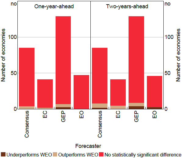
For the vast majority of economies, we find no statistically significant difference at a 5 per cent level in forecast accuracy (Figure 1). For the one-year horizon there are a handful of economies where Consensus and EC are found to outperform or underperform WEO, and at the two-year horizon there are a few economies where each forecaster outperforms or underperforms.
Note: Test uses 5 per cent level of significance.
Sources: Authors' calculations; Consensus Economics; European Commission; IMF; OECD; World Bank.
Since we perform DM tests separately for dozens of economies with a 5 per cent level of significance, even if the null hypothesis is true we would expect around 5 per cent of economies to show a significant result. This would be just two or three economies for EC, EO and Consensus, and zero or one economies for GEP. Hence, the handful of economies with statistically significant differences could be spurious. If one of the forecasters was genuinely better or worse in general, we would expect to see that forecaster outperform or underperform for many economies, but this is not the case. The results for each individual economy at a one-year-ahead horizon are available in Table B.1.
The lack of significant results could occur because there is genuinely no meaningful difference in performance, or because our sample sizes are too small to detect any performance differences. Our paper benefits from having access to more recent forecast vintages than earlier studies, increasing the power of our tests (see Section 2.1). Nevertheless, the sample sizes are modest. This is especially true for comparisons of GEP or EC, whose forecast vintages start in 2010 and 2011 respectively.
4.2.2 Cross-economy evidence
The hypothesis tests considered each economy in isolation. A natural question is whether one can better detect differences in forecast performance by drawing on the results for many different economies. Unfortunately, it is not straightforward to use the observed performance for different economies in a formal hypothesis test. The reason is that actual outcomes are correlated across economies (e.g. high growth in France tends to coincide with high growth in Germany), and forecasts tend to be correlated across economies too (e.g. if the IMF expects high growth in the United States it likely expects high growth in Mexico too). As such, the forecast errors for different economies do not provide independent sources of information.
Nevertheless, considering the results for many economies together provides suggestive evidence for differences in performance between forecasters. This suggests that, while tests of differences in forecast accuracy typically fail to reject the null at present (Section 4.2.1), future studies with longer sample periods may find differences more often.
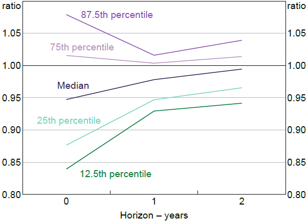
First we compare Consensus to WEO. For each horizon, we sort economies from the lowest ratio of Consensus RMSFE to WEO RMSFE to the highest. At zero or one-year horizon, roughly 75 per cent of economies had a lower Consensus RMSFE than WEO RMSFE (Figure 2). This provides suggestive evidence that Consensus mean forecasts are more accurate than WEO in general. Of course, absent a formal hypothesis test, we cannot say how likely it is that Consensus outperformed WEO by this much over the sample period simply by chance. If the Consensus mean is more accurate in general, it might reflect that combining forecasts of different forecasters tends to improve accuracy (e.g. Clements and Harvey 2009).
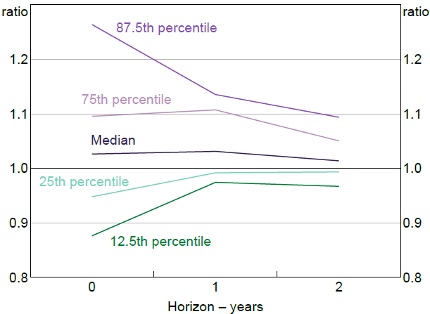
Second, we compare EO to WEO using the same exercise. At a one-year horizon, around 75 per cent of economies had a higher EO RMSFE than WEO RMSFE (Figure 3). This suggests WEO may be more accurate than EO in general. This cannot be attributed to differences in the timing with which each forecaster publishes their forecasts, because although the EO has a one month timing advantage in some vintages, it has a one month timing disadvantage in other vintages (Table 2).
We also compare both EC and GEP to WEO. These do not have a clear pattern in either direction. These point estimates are noisier, as the comparisons are based on a smaller set of vintages than EO or Consensus.
Sources: Authors' calculations; Consensus Economics; IMF.
Sources: Authors' calculations; IMF; OECD.
4.3 Decomposing differences in forecast performance
A loss differential measures the difference in accuracy of two forecasts for the same outcome. We show that in the case of squared error loss, a loss differential can be decomposed into two components: the accuracy of the average forecast and the disagreement between forecasters. This decomposition can be applied to any comparison of pairs of forecasters, as it is not specific to a particular variable (such as real GDP growth) or a particular type of forecaster (such as international organisations).
Theorem 1. Suppose the loss differential between a forecaster c and another forecaster b is computed with squared error loss:
Then the absolute loss differential can be written:
Proof. See Appendix B.1.
If we assume that the loss differential, the error in the average forecast, and the absolute difference in forecasts are all non-zero, we can take natural logs, giving:
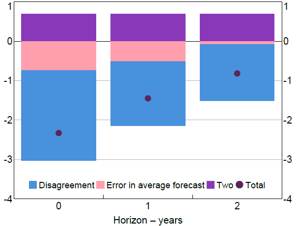
Before taking logs, we omit observations for which the absolute loss differential or either component is less than 0.01. We can use this decomposition to understand how the relative performance of a pair of forecasters for an economy depends on the forecast horizon. To do this, we compute sample means of the log absolute loss differentials across all forecast dates, and sample means of the components.[15] Figure 4 shows this decomposition for the Consensus and WEO forecasts for the United States. At longer horizons, the log absolute loss differential is less negative, which means the absolute loss differential is larger. Our decomposition shows that this occurs because longer horizons have both larger amounts of disagreement and larger errors in average forecasts.
The decompositions for individual economies are not too informative in our application. As discussed in Section 4.2.1, we find statistically significant differences in accuracy for only a few economies, possibly reflecting the modest sample sizes of forecasts. However, the decompositions for individual economies may be informative in future studies with larger sample sizes, including studies on other variables or types of forecaster.
Sources: Authors' calculations; Consensus Economics; IMF.
We also consider the results for many economies together, as this may reveal patterns that are hard to detect for individual economies. To do this, we perform the decomposition for each individual economy, and then summarise the results by estimating a panel regression (Equation (2)). The dependent variable is the log absolute loss differential for a particular economy i, forecast month t and horizon h. The explanatory variables are economy fixed effects and dummies for each horizon. We include a horizon dummy for each horizon h = 1,...,H, which means the base case is a horizon of h = 0 years.[16] The economy fixed effects are included because the magnitude of loss differentials is likely to differ across economies.[17]
We then perform two more panel regressions with the same explanatory variables, but where the dependent variable is a term from our decomposition (Equation (3)).
Figure 5 shows the estimated coefficients on the horizon dummies for the comparison of Consensus to WEO. Figures 6, 7 and 8 do the same for comparisons involving EC, GEP and EO respectively. Across all four pairs of forecasters, we find that, relative to the zero-year-ahead base case, the log absolute loss differentials are larger at a one-year horizon, and larger still at a two-year horizon. Our results show that, over the sample period, this occurred because the errors in the average forecast were larger at longer horizons, and to a lesser extent, because disagreement between the forecasters was larger at longer horizons. Whether this is true in the population is hard to assess.[18] It makes sense that the forecast errors and disagreement are both larger at longer horizons, since forecasters have less information at these horizons. In particular, the forecasts at a zero-year horizon typically benefit from having data for some quarters of the year.
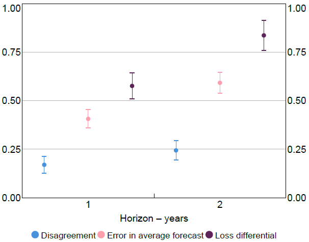
Note: Whiskers show 95 per cent confidence intervals.
Sources: Authors' calculations; Consensus Economics; IMF.
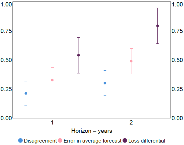
Note: Whiskers show 95 per cent confidence intervals.
Sources: Authors' calculations; European Commission; IMF.
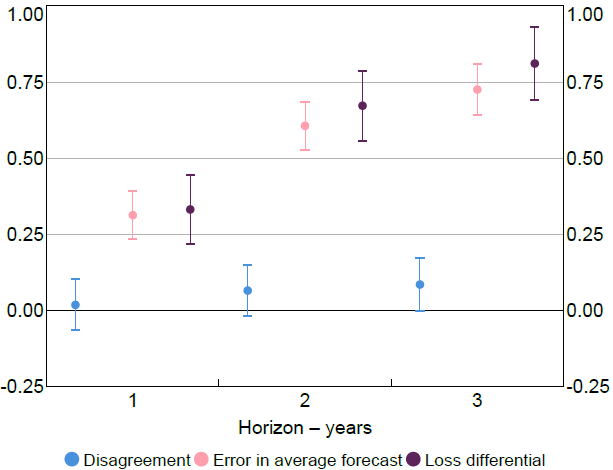
Note: Whiskers show 95 per cent confidence intervals.
Sources: Authors' calculations; IMF; World Bank.
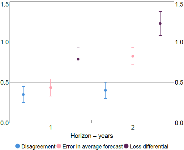
Note: Whiskers show 95 per cent confidence intervals.
Sources: Authors' calculations; IMF; OECD.
Our results suggest that practitioners should be cautious when interpreting the size of loss differentials at different horizons: if the difference in squared errors becomes larger in magnitude at longer horizons, this does not necessarily indicate changes in the relative performance of the two forecasters, but rather could arise simply because both forecasters are less accurate at longer horizons.
5. Testing Forecast Rationality
5.1 Methods of testing forecast rationality
We perform rationality regressions on fixed-horizon forecasts to test the joint assumption of rationality and squared error loss. Specifically, we test the null that the parameter vector is the zero vector in Equation (1).
The key assumption is that the error in this regression is covariance stationary.[19] However, we allow for the possibility that the error in this regression is heteroskedastic and autocorrelated.[20] Under our assumptions, the OLS estimator of is asymptotically normal, so we can perform asymptotically valid t-tests and Wald tests of hypotheses concerning using a HAC estimator of the covariance matrix of the OLS estimator (see the introduction of Kiefer et al (2000)). We use the HAC estimator in the ‘sandwich’ package in R with the default options (Zeileis 2004), just as we did in the DM tests.
Our rationality test raises similar econometric issues to the DM test (as discussed in Section 4.1), which is to be expected given that both are tests about the coefficients of a regression involving forecast errors. Firstly, the test has an asymptotic justification, but as with any evaluation of macroeconomic forecasts, we only have modest sample sizes. This problem is less severe here than some other papers, as our sample includes recent forecast vintages that were unavailable to researchers in previous years. Secondly, the forecasts may be produced using explicit models that are estimated on finite samples, or using judgement that is informed by finite samples. Some authors, such as West and McCracken (1998), have shown that even in the presence of parameter estimation error, one can test hypotheses about the forecast errors that would arise absent that error. However, we are not able to conduct such an exercise as there is no single explicit model for each forecaster. Hence we do not try to account for estimation error in model parameters, following Rossi and Sekhposyan (2016).
In brief, we find that international organisations' growth forecasts fail rationality tests for most economies. The source of the failure of the test varies by economy. In many cases, it arises because the forecasts are too extreme, the forecast revisions are too large, or the forecasts have an optimistic bias.
5.2 Regression specifications
5.2.1 The general specification
Our general regression specification is:
This regression includes the following elements:
- The dependent variable, , is the error in the forecast for period (t + h) made in period t.
- The forecasts for the target year. This includes the forecast that was used to compute the error, , and one earlier forecast, .
- Errors in h-step-ahead forecasts. We let p denote the number of periods it takes for statistical agencies to publish the actual real GDP growth outcome after the end of a period. This implies that, in period t, the latest actual known to the forecaster is . Our regression includes the latest forecast error known to the forecaster, , and one earlier error, .
In the notation of Equation (1), the vector xt comprises the intercept, forecasts for the target year and errors in h-ahead forecasts, and the vector of parameters is . The rationality test is a Wald test of against .
It would be straightforward to add more lags of forecasts or errors to this regression. We choose not to, as it may result in the parameters being estimated very imprecisely given the modest sample sizes of macroeconomic forecasts available.
When we estimate these regressions, we are careful to ensure the regressors only reflect information available to the forecaster at the time. For example, in one observation in this dataset, the dependent variable is the error in the April 2020 WEO forecast for 2022. The regressors include two forecasts for that target year: the April 2020 WEO forecast for 2022, and the January 2020 WEO forecast for 2022. Both of these forecasts would have been known to the IMF at the time. The regressors also include two errors in two-year-ahead forecasts. As of April 2020 WEO, if the most recent actual for a particular economy is 2019, the two latest two-year-ahead errors are the error in the April 2018 forecast for 2019 and the error in the April 2017 forecast for 2018. These two errors are computed with the April 2020 vintage of actuals, rather than the latest vintage.[21]
5.2.2 Interpreting the general specification
Interpreting the parameters of the rationality regression is difficult. In particular, the intercept is not the forecaster's unconditional bias, but rather is the bias conditional on past forecasts and past errors all being zero. To facilitate interpretation, it is useful to rearrange Equation (4) as follows.[22]
The right-hand-side terms each have a nice interpretation.
- The first term is the unconditional bias, which is the expectation of the forecast error. This differs from the intercept, which is the conditional bias given that all the explanatory variables are zero.
- The contribution of demeaned forecasts tells us if the forecasts tend to be ‘too extreme’ or ‘not extreme enough’. For example, suppose the coefficient on the latest forecast is positive . If the forecaster predicted higher growth than they usually do, , then the forecast error is likely to be positive, , so the forecast error would have been smaller if the forecast were even higher. Conversely, if the forecaster had predicted lower growth than usual, the forecast error would likely be negative, so the forecast error should have been even lower. For this reason, we describe as indicating that the jth most recent forecast was not extreme enough, and as indicating that it was too extreme.
- The contribution of demeaned forecast errors tells us if the forecaster's h-period-ahead errors are related to the latest h-period-ahead-errors known on the forecast date, which would indicate that the forecaster is not making efficient use of the information contained in their past errors. For example, the forecaster may be slow to recognise that a change in the mean of the series has occurred, and hence persistently overpredict growth over a long period.
We cannot estimate the rearranged regression directly, because this would require knowledge of the population mean of forecasts and the population mean of errors. Instead, we estimate the original regression (Equation (4)), but we bear the rearranged regression in mind when interpreting the coefficients. Since we cannot estimate the rearranged regression directly, we cannot use it to test the hypothesis of zero unconditional bias. Instead, we need to estimate a regression of errors on an intercept alone, as in Section 5.3.3.
5.3 Results
5.3.1 General specification
We perform a Wald test of the null hypothesis of forecast rationality (all parameters equal zero) against the alternative of irrationality. For most forecasters, we reject rationality of one-year-ahead and two-year-ahead forecasts at a 5 per cent level for most economies (Figure 9). The exception is EO, where we only reject rationality for half of economies at one-year-ahead and a minority of economies at two-years-ahead. The samples of forecasts available for EO are smaller than for WEO and Consensus, which reduces the power of tests for EO.
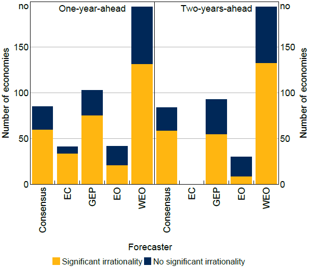
Notes: Test uses 5 per cent level of significance. The sample of two-years-ahead EC forecasts is small, so this series is not shown.
Sources: Authors' calculations; Consensus Economics; European Commission; IMF; OECD; World Bank.
Having found widespread irrationality, we now investigate the source of irrationality. First, we perform Wald tests of the null that the coefficients on past forecasts are zero, which we reject for most economies (Figure 10). As explained in Section 5.2.2, this indicates that the forecasters have a tendency to make forecasts that are too extreme or not extreme enough.
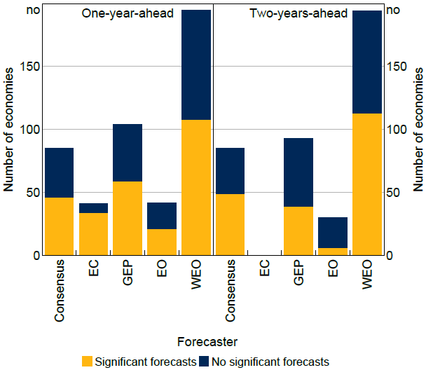
Notes: Test uses 5 per cent level of significance. The sample of two-years-ahead EC forecasts is small, so this series is not shown.
Sources: Authors' calculations; Consensus Economics; European Commission; IMF; OECD; World Bank.
Second, we perform Wald tests of the null that the coefficients on past errors are zero. Some forecasters, including the IMF, OECD and EC, only review their forecast performance every few years (Genberg et al 2014), so it is plausible that they would fail to make efficient use of any of the information contained in their recent errors. We reject the null that the coefficients on past errors are zero for a minority of economies (Figure 11). Since we conduct a separate hypothesis test at the 5 per cent level for each economy and forecaster, we would expect the Wald test to be rejected for 5 per cent of economies if the null hypothesis were true for all economies. These results provide tentative evidence that a failure to make use of the information in past errors is a source of irrationality for some forecasters for some economies, but suggest this issue is not too widespread.
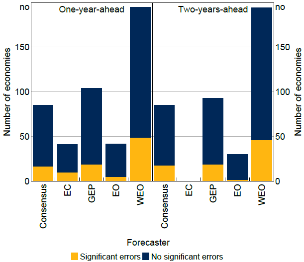
Notes: Test uses 5 per cent level of significance. The sample of two-years-ahead EC forecasts is small, so this series is not shown.
Sources: Authors' calculations; Consensus Economics; European Commission; IMF; OECD; World Bank.
5.3.2 Intercept and past forecasts specification
The Wald tests of the general specification suggest that failing to account for information in past errors is a relatively unimportant source of irrationality. For this reason, we consider a special case of the general specification where these past errors are removed:
We can view this regression through the lens of forecast revisions, which are changes in forecasts for a given target year from one vintage to the next. We rearrange the specification with forecasts only to obtain a specification with a forecast revision and a past forecast (Equation (7)).
The coefficient on the latest forecast revision tells us if the forecast revisions tend to be too large or too small. For example, if , it implies that if the forecaster revised up their forecast in the last period, , then the forecast error is likely to be positive, , which implies that the forecast error would be smaller if the upward forecast revision had been larger. Hence whenever we say that the latest forecast revision tends to be too small, indicating that the forecaster tends to underreact to the news received between t – 1 and t.[23]
We test rationality in Equation (7) by performing a Wald test of the null that all coefficients are zero (Figure 12). We reject rationality for many.
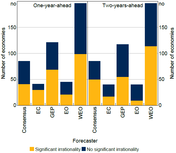
Note: Test uses 5 per cent level of significance.
Sources: Authors' calculations; Consensus Economics; European Commission; IMF; OECD; World Bank.
We know that this irrationality is not solely due to bias, because if we do a Wald test of the coefficient on the revision and on the past forecast, we reject the null for the majority of economies for all forecasters. To understand the role of revisions versus past forecasts, we do t-tests of each, noting that for some economies neither variable may be individually significant even though the two variables are jointly significant.
The t-tests of the coefficient on the past forecast show that this coefficient is insignificant in most economies (Figure 13). Where the t-tests are significant, the forecasts are typically too extreme. When the forecaster expects higher-than-average growth, they could improve accuracy by making a less optimistic forecast, and when the forecaster expects lower-than-average growth, they could improve accuracy by making a less pessimistic forecast. Halperin and Mazlish (2025) find, using regressions that pool across economies, that Consensus mean forecasts are too extreme. Their finding is consistent with our results, which show that Consensus mean forecasts are too extreme for a sizable minority of economies.
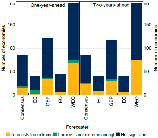
Note: Test uses 5 per cent level of significance.
Sources: Authors' calculations; Consensus Economics; European Commission; IMF; OECD; World Bank.
The t-tests show that the coefficient on revisions is significant in many economies (Figure 14). However, the direction of the inefficiency differs. In each international organisation, it is more common for revisions to be too large than for them to be too small. This is similar to the finding that individual private-sector forecasters make overly large forecast revisions (Bordalo et al 2020; Broer and Kohlhas 2024). For the average of Consensus forecasts, it is more common for revisions to be too small, consistent with previous evidence that the average of private-sector forecasts has overly small forecast revisions (Coibion and Gorodnichenko 2012, 2015). However, our finding contrasts with Halperin and Mazlish (2025), who find that average private-sector forecasts for real GDP have overly large revisions at horizons of two or more years.
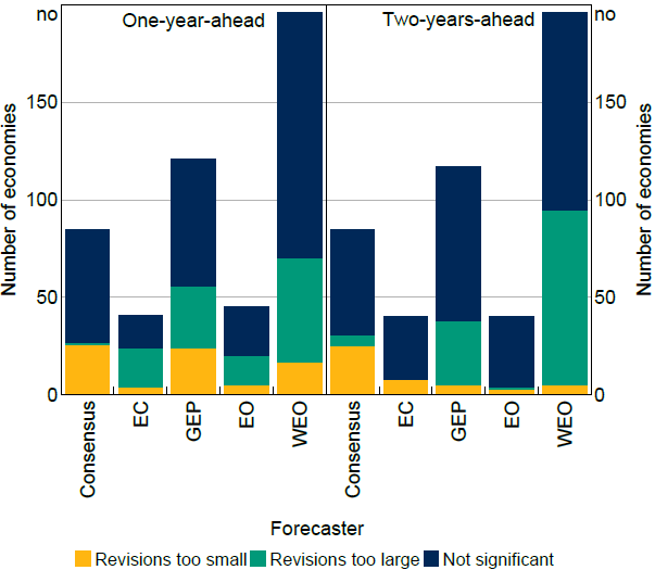
Note: Test uses 5 per cent level of significance.
Sources: Authors' calculations; Consensus Economics; European Commission; IMF; OECD; World Bank.
An alternative to regressing errors on forecasts (as we have just done) would be to regress forecast revisions on their own lags. Nordhaus (1987) shows that if forecasters incorporate all new information each time they update their forecasts, then the sequence of forecast revisions for a fixed target date will be serially uncorrelated. Such a sequence of forecast revisions is said to satisfy ‘weak efficiency’, which is a necessary condition for rationality. Hadzi-Vaskov et al (2021) find, using WEO real GDP growth forecasts, that the sequence of revisions for a given target year are negatively autocorrelated. This is consistent with our finding that WEO revisions are too large for a sizable minority of economies.
5.3.3 Intercept only specification
We also estimate a specification with the intercept alone. By doing this we are not claiming that the revision and past forecast are absent from the true model. As we saw earlier, the forecast revision and past forecast are jointly significant in most economies. Rather, we estimate this specification so that we can test for unconditional bias by performing a t-test of the intercept, as is standard in the literature. Although we could provide point estimates of unconditional bias in each economy using the previous specifications, we were not able to formally test if it was equal to zero.
For all forecasters, we find that there is no significant unconditional bias for most economies at the one-year or two-year horizon (Figure 15), though bias is more common at a two-year horizon for GEP and WEO. Where bias is present, it is almost always optimistic rather than pessimistic.
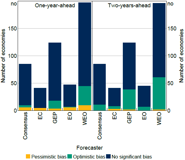
Note: Test uses 5 per cent level of significance.
Sources: Authors' calculations; Consensus Economics; European Commission; IMF; OECD; World Bank.
To summarise, we have shown that international organisations' growth forecasts fail rationality tests for the majority of economies. The reason for the rejection of this test differs by economy, but common reasons are that the forecasts are too extreme (Figure 13), revisions being too large (Figure 14), and optimistic bias (Figure 15).
6. Explanations
In Section 5, we conducted rationality tests for the forecasts from international organisations and Consensus by regressing forecast errors on an intercept, past forecasts for the target year and past forecast errors. Where the null hypothesis of the rationality test is false, then at least one of the following must be true:
- the forecaster does not satisfy forecast rationality;
- the forecaster must not have a squared error loss function; or
- the vector of explanatory variables, xt must not be in the forecaster's information set.
If the null is false then this is likely because the forecaster does not satisfy forecast rationality or does not have squared error loss, rather than because the explanatory variables are absent from their information set. The reason is that the explanatory variables in our regressions are the forecaster's own forecast or the errors in their own forecasts, which are almost certainly known to the forecaster.
An extensive literature provides explanations for why different types of agents, such as consumers or firms, may make irrational forecasts. However, the explanations for irrationality at international organisations may be quite different, given that they make forecasts using different methods and face different incentives. In this section we consider two explanations that are based on specific features of international organisations:
- International organisations make forecasts that are conditional on assumed future values of a variety of explanatory variables. Such forecasts violate forecast rationality under fairly general conditions (Section 6.1).
- International organisations may report a ‘modal’ forecast, rather than a mean forecast (Section 6.2).
6.1 Conditioning assumptions
6.1.1 The rational expectations approach
Future growth,
By the law of iterated expectations, this rational forecast equals:
That is, the forecaster can make a rational forecast by:
- Computing a conditional expectation of future growth given a value of the future explanatory variables, , for each possible value of the explanatory variables; and then
- Averaging this conditional expectation, , over the various possible paths of the explanatory variables, weighted by the conditional probabilities of each possible value of the explanatory variables given the information set.
For example, one would compute the expected path for growth for each possible scenario for crude oil prices, and then compute a weighted average of those different paths for growth weighted by the likelihood of each crude oil price scenario.
6.1.2 The current approach at international organisations
International organisations make forecasts that are conditional on assumed future values of the explanatory variables.
In each WEO, the IMF publicly states its assumptions for exchange rates, oil prices, bond yields, monetary policy and fiscal policy. In addition, the IMF makes assumptions about other issues on an ad hoc basis. In the April 2021 WEO, for instance, the IMF made assumptions about COVID-19 vaccination and testing (IMF 2021).
The EC and OECD follow a similar practice of making assumptions about future explanatory variables such as exchange rates and then making growth forecasts conditional on those assumptions (Genberg et al 2014). Though central banks don't form part of our dataset, it's worth noting that they follow this practice as well (e.g. Kohler 2023). It's unclear what practices private-sector forecasters follow, as their forecasting processes are rarely as well documented publicly as those of international organisations.
6.1.3 Current practice typically differs from rational expectations
We will use the term ‘current practice’ forecast to refer to the conditional expectation of future growth conditional on an assumed future value of the explanatory variable .
Current practice will typically be inconsistent with rational expectations. This is true whether the assumed values of the explanatory variables are rational forecasts or not. We will consider each case in turn.
Case with rational forecasts for explanatory variable
First, suppose that the forecaster's assumed future value of the explanatory variable is a rational forecast for that variable, . Then the current practice forecast will be:
Whether the current practice forecast of growth coincides with the rational forecast depends on two factors. Firstly, what is the relationship between future growth and the future explanatory variable? This relationship is described by the ‘response function’, . Secondly, what is the conditional distribution of the future explanatory variable given the information set? This is described by the conditional probability density function (pdf) .
The next theorem provides sufficient conditions for the current practice forecasts to be rational. For simplicity, the theorems and proofs consider a scalar explanatory variable. They condition on a fixed information set, omit that information set and the time subscripts from the notation, and denote . We assume that and are finite.
Theorem 2. The rational forecast will equal the current practice forecast if:
- the response function r is affine, that is, for constants a and b; or
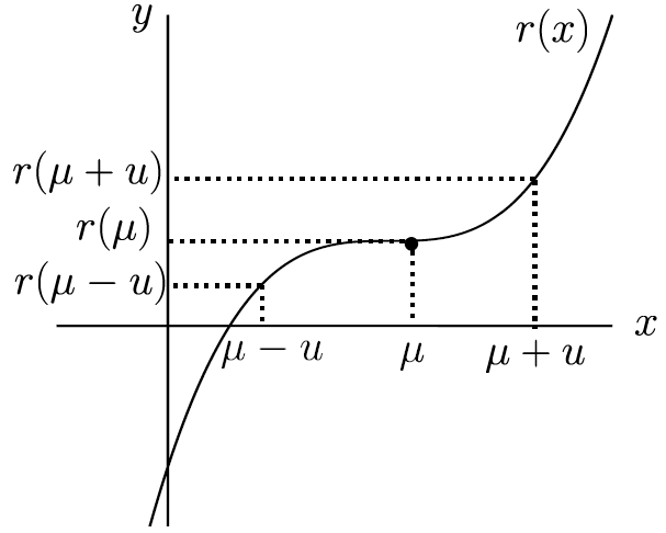
- the response function r has 180 degree rotational symmetry about the point , and the conditional pdf p is symmetric about its mean, .
Proof. See Appendix C.
To give intuition for the theorem, the rational forecast of y considers the possibility that x could be above its mean and that x could be below its mean. Under the assumptions of this theorem, these two considerations have exactly offsetting effects, so the rational forecast coincides with the current practice forecast, which assumes that x will equal its mean. Consider case (b) where r satisfies the rotational symmetry assumption. As illustrated by Figure 16, if the explanatory variable is a distance u above its mean, the response function would change by . If the explanatory variable were the same distance below its mean, the response function would change by . The rotational symmetry assumption states that these two changes are the same in size and opposite in sign.
Since the future explanatory variable has a symmetric distribution about its mean, it is just as likely to be above its mean by u units as below its mean by the same amount. Hence, the rational forecast equals the current practice forecast.
If either of these symmetry conditions fail, then the current practice forecast may differ from the rational forecast, as we now show.
Theorem 3. Suppose the future explanatory variable has a non-degenerate distribution.
- If the response function r attains a strict global minimum (maximum) at the rational forecast for the explanatory variable, , then the rational forecast will be strictly greater than (strictly less than) the current practice forecast.
- If the response function r is strictly convex (strictly concave), then the rational forecast will be strictly greater than (strictly less than) the current practice forecast.
Proof. See Appendix C.
To illustrate, consider the dependence of real GDP growth on rainfall, which may be important in low-income economies where agriculture is a large share of GDP. Typically, the kinds of agriculture undertaken in a given location are those that provide high yields when rainfall is typical for that location. For example, rice in areas with high rainfall and wheat in areas with lower rainfall. Hence it may be approximately correct to assume that real GDP growth in a low-income economy attains a strict global maximum at the average level of rainfall, or that growth is strictly concave in rainfall. If either of these assumptions is true, Theorem 3 implies that the rational forecast will be lower than the current practice forecast.
Case with irrational forecasts for explanatory variables
The preceding discussion assumed that the assumed future values of the explanatory variables are rational forecasts for those variables. This is likely to be approximately true when those assumptions are based on financial markets, as when crude oil price assumptions are taken from crude oil price futures. However, when assumptions are made in other ways they may be far from rational forecasts.
Assumptions about future fiscal policy will often differ greatly from rational forecasts. Where the IMF or EC are providing financing to an economy, they assume that the economy will fully implement any policies it agreed to as a condition of the financing (Genberg et al 2014). It is unlikely that expecting full compliance is a rational forecast, given that economies often comply only in part. For other economies, the IMF and EC approach:
assumes that policy changes will occur during the forecast period only if they have been legislated in advance or if there is substantial knowledge that suggests they will occur. Otherwise, policy is assumed to remain constant during the forecast period. (Genberg et al 2014, pp 35–36)
This is also unlikely to be a rational forecast, as it ignores the systematic tendency of governments of advanced economies to vary their fiscal policy to smooth out business cycle fluctuations.
6.2 Modal forecasts
6.2.1 Which forecasters make modal forecasts?
For a given conditional distribution of future growth, a forecaster could report the mean, the mode, the median, or some other summary statistic. Surveys of professional forecasters typically do not specify the type of point forecasts respondents should provide. For example, Elliott et al (2008) notes that the US Survey of Professional Forecasters does not specify the type of point forecasts that respondents should provide. Similarly, international organisations refer to their forecasts using vague terms such as ‘central forecast’.
It's likely that at least some international organisations see themselves as making modal forecasts. One piece of evidence is that some major central banks make modal forecasts.[24] This suggests international organisations may do the same, given that they use similar forecasting models, are staffed by economists with similar training, and follow similar internal processes during forecasting rounds.
Some private-sector forecasters may also see themselves as making modal forecasts. This view was held, for instance, by JP Morgan (Davies 2017).
6.2.2 How would modal forecasts affect rationality tests?
Consider a forecaster who is able to compute the conditional distribution of growth given the information available on the forecast date.
- The forecaster could report the conditional expectation of growth, . In this case, their forecasts would satisfy rationality tests. That is, their forecast errors would be orthogonal to any vector of known variables xt (see Equation (1)).
- If the conditional distribution is unimodal, the forecaster could instead report the conditional mode of growth, . If the conditional distribution is also symmetric, then the mode would coincide with the mean, and these forecasts would satisfy rationality tests. However, if the conditional distribution is asymmetric, the mode could differ from the mean, and the forecasts may not satisfy rationality tests.
Modal forecasts may fail rationality tests due to bias (as recognised in Kangur et al (2019)). However, modal forecasts may also fail rationality tests due to correlations of forecast errors with other explanatory variables (which has not been recognised previously). Biased forecasts will cause the rejection of rationality tests whenever the vector xt includes a constant, because the bias would lead to the coefficient on that constant being non-zero. As shown in Bekaert and Popov (2019) and Burgess et al (2021), past growth outcomes have been negatively skewed in most economies. If the conditional distribution of future growth given the forecaster's information set is also negatively skewed, then the mode will often exceed the mean, in which case modal growth forecasts will have an optimistic bias.
Modal forecasts may result in correlations between forecast errors and other explanatory variables. For example, suppose that growth is a realisation from one of two non-overlapping distributions: a ‘crisis’ distribution centred on –5 per cent, or a ‘non-crisis’ distribution centred on 2 per cent. Let the probability of a crisis next year be low. Assume that the conditional mode remains the mode of the non-crisis distribution even if the crisis probability varies. The mean will then depend on both distributions, while the mode will depend only on the non-crisis distribution. Suppose some variable in xt, such as the debt-to-GDP ratio, is positively correlated with the probability of a crisis next year. Then that conditional expectation of growth will be a decreasing function of that variable, while the conditional mode of growth will be unrelated to that variable. This implies that, if the forecaster makes a modal forecast, their resulting forecast errors will be negatively related with that variable, causing the failure of rationality tests.
6.2.3 Empirical evidence on whether making modal forecasts introduces bias
We have just argued that the practice of making modal forecasts could result in biased forecasts. We now show empirically that modal growth outcomes tend to exceed mean growth outcomes, which suggests that this bias might arise in practice, but the effect is small. We also raise a methodological limitation that affects both our method and the similar method of Burgess et al (2021). Due to this limitation, it remains possible that making modal forecasts contributes greatly to bias or not at all.
Conceptual overview of method
Suppose that for any given economy and forecast horizon, the conditional mode for a period t equals the sum of a constant , the conditional mean , and a mean-zero error et.
The constant is the expected difference between conditional mode and mean. This parameter determines whether a hypothetical forecaster that knew the conditional distribution of future growth would make biased forecasts if they reported the conditional mode rather than the conditional mean. Our aim is to estimate this parameter, so our empirical strategy is focused on growth outcomes (which are relevant to the hypothetical forecaster) rather than on the growth forecasts of any particular organisation.
Ideally, we would compute the mean and mode of the conditional distribution of future growth for a sample of periods. Using this sample, we could estimate Equation (8), giving us an estimate of the amount of bias that modal forecasting causes for that economy, . We could also test the hypothesis that modal forecasting does not introduce bias, , against the alternative that it does.
Unfortunately, we do not observe the conditional distribution of growth given particular information sets. Rather, we observe a set of growth outcomes, which provides information about the unconditional distribution of growth. Hence, we need to use our model of conditional distributions (Equation (8)) to make a prediction about unconditional distributions. We do this by taking expectations of Equation (8) over possible information sets.[25]
We then make the further assumption that the unconditional mode, Mode[yt], equals the expectation of the conditional modes, . This assumption is a limitation of the method, as discussed below. With this assumption:
Given a sample of growth outcomes, we would like to estimate the unconditional mode and the unconditional mean, as the difference between them would provide an estimate of . A challenge is that an economy's growth may be a non-stationary process, so its mean and mode may vary over time. For example, some east Asian economies such as Japan experienced high ‘catch-up’ growth followed by more moderate growth. To allow for this, we assume that an economy's growth is the sum of a deterministic component, bt, and a stationary stochastic component, zt.
Substituting this into Equation (9), and recognising that deterministic components can be taken outside of the mode or expectation operator, we have:
Hence, to estimate how much making modal forecasts introduces bias, , we compute the estimated mode of detrended growth less the sample mean of detrended growth. This is somewhat similar to Burgess et al (2021), who compare the sample mean of detrended growth to the sample median of detrended growth.
Implementation and results
We use annual real GDP growth data from the WEO database for all economies whose time series has at least 40 observations. To estimate the stochastic component, we convert the growth rates into log levels, compute detrended log levels, and then compute growth rates of the detrended log levels. We detrend log levels using a two-sided Hodrick-Prescott filter (Hodrick and Prescott 1997), with the parameter value , following the recommendation for annual data given by Ravn and Uhlig (2002). Figure 17 compares actual growth rates, yt, and our estimates of the stationary stochastic component, zt, for Japan.
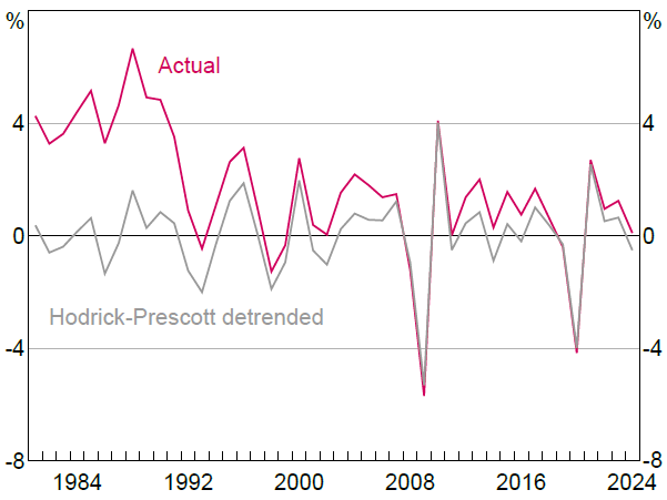
Sources: Authors' calculations; IMF.
We estimate the mode of detrended growth using the half-sample mode estimator as implemented by the ‘modeest’ R package (Poncet 2019). This estimator assumes that the data are drawn from a continuous unimodal distribution, but does not require the assumption of any specific parametric distribution, and has the advantage of being insensitive to outliers (Bickel and Frühwirth 2006). We estimate the mean of detrended growth using the sample mean.
We find that 91 of 145 economies have an estimated mode above the sample mean. These differences are small in magnitude however. On average across all 145 economies, the estimated is 0.16 percentage points.
As a robustness check, we also compute the sample skewness of detrended growth for each economy:
Skewness is important because if the distribution of the detrended growth is unimodal, then its mode will typically exceed its mean when the distribution is negatively skewed. We find that 107 of 145 economies have negative sample skewness. This supports our finding that the unconditional mode exceeds the unconditional mean in most economies. Without this complementary evidence, one might have wondered if our results were driven by the specifics of our mode estimator.
Limitations
Our method assumes that the unconditional mode, Mode [yt], equals the expectation of the conditional mode, . This assumption holds exactly if the conditional mode does not vary with respect to variables in the information set. This is possible in principle. Returning to the example of a crisis introduced above, suppose that a crisis is very unlikely when the debt-to-GDP ratio (the variable entering the information set) is low and that a crisis is somewhat unlikely when the debt-to-GDP ratio is high. For both values of the debt-to-GDP ratio, the crisis will probably not occur, and the conditional mode of growth does not vary with respect to the variable in the information set.
It is more likely, however, that the conditional mode of growth does vary with respect to the information set. In this case, the assumption may or may not hold. We will illustrate this in the extreme case where the information sets fully determine growth. Suppose that there are three possible information sets: ‘pre-bust’, ‘ordinary’ and ‘pre-boom’, which guarantee that growth will be –2, 2 or 6 per cent respectively. First we consider the symmetric case, where ‘pre-bust’ and ‘pre-boom’ each occur with probability and ‘ordinary’ occurs with probability . In this case, the assumption holds:
In practice, business cycles are likely to be asymmetric. Suppose that the probability of ‘pre-bust’ is , of ‘ordinary’ is and of ‘pre-boom’ is 0. Then:
As this discussion illustrates, unconditional modes may differ from the expected conditional mode in the face of asymmetric business cycles, which is a situation we are interested in. Hence, one should be cautious about the results of our method (which suggest that modal forecasts may contribute slight optimistic bias), but also about any other effort to explain forecast bias using the unconditional distribution of growth. In particular, comparing the sample median and sample mean of growth as in Burgess, Langendorf, Ippolito and Pielke (2021) provides an unbiased estimate of the difference between the conditional median and conditional mean only if one assumes that , which is subject to an analogous critique.
7. Conclusion
This paper provides new evidence and theory concerning real GDP forecasts by international organisations. The paper begins by comparing the forecast accuracy of four international organisations and the average of Consensus forecasts, finding statistically significant differences for only a few economies. It presents a new decomposition of differences in accuracy into contributions of disagreement and the accuracy of the average forecast. This decomposition is then used to show that, on average across economies, differences in accuracy are larger at longer forecast horizons due to both greater disagreement and lower accuracy of the average forecast. We then turn to forecast rationality. For most forecasters, we reject the null of the rationality test for most economies. Often the irrationality takes the form of optimistic bias, overly large revisions or forecasts that are too extreme. Finally, we contribute to the literature that attempts to explain why rationality is often rejected in these tests. We focus on two explanations: the use of conditioning assumptions and the practice of making modal forecasts.
Our findings have important implications for the practices of international organisations. Firstly, we find that the international organisations are quite similar to one another in terms of accuracy and the ways in which they fail rationality tests. Secondly, our findings highlight the importance of forecasters being transparent, including about their conditioning assumptions and whether they see themselves as making modal forecasts. This will assist users in interpreting the forecasts. Knowing that a forecaster is making modal forecasts, for instance, will tell users that they should not view the forecasts as incorporating tail risks like financial crises. Transparency will also make it easier to choose among competing explanations for the failure of rationality tests, which will help organisations determine what actions to take in response.
The lessons of this paper can also be applied to other types of forecasters. For example, one can ask whether differences in the accuracy of different private-sector forecasters are larger at longer horizons, and if so, use our decomposition to assess if this reflects greater disagreement or lower accuracy. Or one can investigate the effects of making conditioning assumptions or modal forecasts at central banks or fiscal authorities.
Appendix A: Detail on Data
A.1 Computing forecast horizons
We define the horizon of a forecast as the number of days from the publication date of the forecast to the end date of the target year. The publication date of a forecast is assumed to be the 15th day of the publication month.[26] International organisations and Consensus forecast real GDP growth in calendar years for most economies, but forecast growth in fiscal years in others (see Table A1 for a list). For example, WEO forecasts US real GDP growth in calendar years, so in the October 2019 WEO, the end date of the first target year will be 31 December 2019. However, WEO forecasts Indian real GDP growth in fiscal years, so in the October 2019 WEO, the end date of the first target year will be 31 March 2020.
| Country | WEO | GEP | EO | Consensus |
|---|---|---|---|---|
| Bangladesh | 1 July | 1 July | na | 1 July |
| Bhutan | 1 July | 1 July | na | na |
| Egypt | 1 July | 1 July | na | 1 July |
| Ethiopia | 1 July | 8 July | na | na |
| Haiti | 1 October | 1 October | na | na |
| India | 1 April | 1 April | 1 April | 1 April |
| Iran | 1 April | 21 March | na | na |
| Lesotho | 1 April | 1 January | na | na |
| Marshall Islands | 1 October | 1 October | na | na |
| Micronesia | 1 October | 1 October | na | na |
| Myanmar | 1 October | 1 October | na | 1 October |
| Nauru | 1 July | 1 January | na | na |
| Nepal | 1 August | 16 July | na | na |
| Pakistan | 1 July | 1 July | na | 1 July |
| Palau | 1 October | 1 October | na | na |
| Puerto Rico | 1 July | 1 January | na | na |
| Samoa | 1 July | 1 June | na | na |
| South Sudan | 1 January | 1 July | na | na |
| Tonga | 1 July | 1 July | na | na |
| Uganda | 1 January | 1 July | na | na |
|
Notes: Does not show economies for which all forecasters report real GDP over calendar years. The EC does not produce real GDP growth forecasts for the economies shown in this table. Sources: Consensus Economics; IMF; OECD; World Bank. |
||||
When comparing forecasters or testing the rationality of forecasts, we report results for a set of forecasts with a specific horizon. In the terminology of Clements (1997), we perform ‘rolling event’ regressions rather than ‘fixed event’ regressions, because our regressions are estimated on samples of forecasts with a fixed horizon and a varying forecast date. However, a subtlety is that we round the forecast horizons to ensure we have adequate sample sizes. For example, when we test the rationality of two-year-ahead forecasts by EC, we estimate our regression on all EC forecasts whose horizon in days is between 548 days and 913 days. An alternative to pooling together forecasts with similar horizons is to construct a set of artificial fixed-event forecasts, an approach that has been critiqued by Yetman (2018).
A.2 Computing forecast errors
A.2.1 Source of actual outcomes
For WEO, EO and EC, we compute forecast errors by comparing the institution's forecast with their own actuals. The forecast databases for these institutions provide vintages comprising actual outcomes and forecasts. To distinguish between actuals and forecasts, we need to make an assumption about how long it takes for statistical agencies to publish actual outcomes after the end of the target year. Our assumption is that this takes 90 days. To illustrate, consider WEO vintages of real GDP growth in India. WEO reports Indian real GDP growth over fiscal years that end on 31 March of each year. Growth for fiscal year 2016/17 will be published on 29 June 2017, which is 90 days after the end of the fiscal year. As discussed above, we assume the publication date of a forecast is the 15th day of the publication month. Hence, the June 2017 WEO vintage is assumed to have been published on 15 June 2017, so we assume that the value reported by WEO for 2016/17 is a forecast rather than an actual outcome.
The GEP database also contains both forecasts and actuals, so they need to be distinguished as above. However, the data on actuals has too short a history to enable the calculation of forecast errors. Hence, we compute errors in GEP forecasts by comparing them with WEO actuals. One might be concerned that the forecasts for an economy may be recorded over a different year as the actuals, since they are taken from different sources. Unfortunately, there are some economies for which the GEP forecasts are recorded over different years to the WEO actuals, and we are unable to compute forecast errors in these economies (see Table A1 for the specific economies).
Consensus provides forecasts, but not actuals. Hence, we compute errors in Consensus forecasts by comparing them with WEO actuals. Fortunately, Consensus uses the same years as WEO for all economies where it makes forecasts.
A.2.2 Rationale for use of latest vintage of actual
For all forecasters, we compute errors using the latest vintage of the actual at the time of writing. An alternative approach would have been to take the first vintage of the actual. Revisions to real GDP data can be substantial (Genberg and Martinez 2014a), so this would lead to different results. Our choice of approach rests on two claims:
- International organisations should aim to forecast the best estimate of true real GDP growth. True growth determines other economic variables and welfare, so a forecast for the best estimate of true growth is the best guide to policy.
- Later vintages of actuals are better estimates of ‘true’ growth than earlier vintages. A major source of revisions to real GDP data is that the statistical agency receives additional data over time. For example, a statistical agency may produce the first vintage of a component of GDP based solely on survey data, but produce more accurate later vintages using tax data as well. This makes later vintages better estimates of true growth. Another source of revisions is changes to international and national standards for the measurement of GDP. Whether such revisions also make the data a better estimate of true growth is less clear. One view is that the changed standards better approximate some ideal notion of real GDP. Another view is that the later vintages are estimates of a slightly different variable to that which the forecaster had in mind.[27] In our view, even if one is concerned about changing standards, this second claim would still hold because the later vintages of GDP benefit so much from additional data.
Taken together, these claims imply that international organisations should aim to forecast the latest vintage of the actual, which makes this latest vintage the proper standard by which the accuracy and rationality of their forecasts should be assessed.
A limitation of our approach is that it reduces the comparability of earlier and later errors, since forecasts from earlier vintages will be compared to actuals that have been revised many times, while forecasts from later vintages will be compared to actuals that have been revised only a few times. On balance, however, we judge that it is appropriate to compute errors using the latest vintage of the actuals.
Appendix B: Comparing Accuracy Across Forecasters
B.1 Proof for Section 4.3
Proof of Theorem 1. The loss differential can be given the following multiplicative decomposition:
Hence the absolute loss differential can be decomposed as:
B.2 Estimation method for panel regressions in Section 4.3
We combine Equations (2) and (3) into a single equation by defining a new variable, , where k is one of l (loss differential), e (error in average forecast) or d (disagreement)
Substituting in the constraints gives:
Rearranging gives the following equation. We estimate it with OLS.
Using the OLS estimates of , we compute and . To test a hypothesis about or , we can perform a Wald test of the appropriate restriction on , using a HAC estimator of the covariance matrix of .
B.3 Full results of comparisons of accuracy
| EC | EO | GEP | Consensus | ||||||||
|---|---|---|---|---|---|---|---|---|---|---|---|
| RMSFE ratio | p-value | RMSFE ratio | p-value | RMSFE ratio | p-value | RMSFE ratio | p-value | ||||
| Afghanistan | na | na | na | na | 0.956 | 0.370 | na | na | |||
| Albania | 1.116 | 0.368 | na | na | 0.841 | 0.260 | 0.888 | 0.050 | |||
| Algeria | na | na | na | na | 1.016 | 0.820 | na | na | |||
| Angola | na | na | na | na | 1.049 | 0.456 | na | na | |||
| Argentina | na | na | 0.978 | 0.720 | 1.070 | 0.147 | 0.951 | 0.072 | |||
| Armenia | na | na | na | na | 0.998 | 0.948 | 0.932 | 0.071 | |||
| Australia | na | na | 1.002 | 0.987 | na | na | 0.869 | 0.051 | |||
| Austria | 0.918 | 0.054 | 0.994 | 0.922 | na | na | 0.997 | 0.911 | |||
| Azerbaijan | na | na | na | na | 1.059 | 0.562 | 0.979 | 0.861 | |||
| Bahrain | na | na | na | na | 1.019 | 0.395 | na | na | |||
| Bangladesh | na | na | na | na | 1.263 | 0.234 | 1.050 | 0.566 | |||
| Belarus | na | na | na | na | 1.103 | 0.208 | 1.045 | 0.592 | |||
| Belgium | 1.004 | 0.917 | 0.971 | 0.600 | na | na | 0.956 | 0.348 | |||
| Belize | na | na | na | na | 0.931 | 0.039 | na | na | |||
| Benin | na | na | na | na | 0.999 | 0.988 | na | na | |||
| Bhutan | na | na | na | na | 0.870 | 0.186 | na | na | |||
| Bolivia | na | na | na | na | 1.015 | 0.253 | 1.014 | 0.689 | |||
| Bosnia & Herzegovina | na | na | na | na | 0.947 | 0.776 | 1.053 | 0.193 | |||
| Botswana | na | na | na | na | 1.040 | 0.386 | na | na | |||
| Brazil | na | na | 0.974 | 0.605 | 1.020 | 0.823 | 0.892 | 0.006 | |||
| Bulgaria | 1.231 | 0.083 | 1.167 | 0.169 | 1.153 | 0.067 | 1.012 | 0.735 | |||
| Burkina Faso | na | na | na | na | 0.959 | 0.456 | na | na | |||
| Burundi | na | na | na | na | 0.840 | 0.046 | na | na | |||
| Cabo Verde | na | na | na | na | 1.014 | 0.365 | na | na | |||
| Cambodia | na | na | na | na | 1.012 | 0.347 | na | na | |||
| Cameroon | na | na | na | na | 0.926 | 0.776 | na | na | |||
| Canada | 1.062 | 0.304 | 1.029 | 0.238 | na | na | 0.956 | 0.029 | |||
| Central African Republic | na | na | na | na | 0.116 | na | na | na | |||
| Chad | na | na | na | na | 1.025 | 0.743 | na | na | |||
| Chile | na | na | 1.081 | 0.103 | 1.201 | 0.132 | 0.979 | 0.317 | |||
| China | na | na | 1.570 | 0.277 | 1.102 | 0.352 | 0.955 | 0.246 | |||
| Colombia | na | na | 0.958 | 0.434 | 1.018 | 0.492 | 0.978 | 0.263 | |||
| Comoros | na | na | na | na | 0.839 | 0.354 | na | na | |||
| Congo, Rep of | na | na | na | na | 1.024 | 0.719 | na | na | |||
| Costa Rica | na | na | 1.002 | 0.948 | 0.988 | 0.737 | 0.954 | 0.110 | |||
| Côte d'Ivoire | na | na | na | na | 1.196 | 0.131 | na | na | |||
| Croatia | 0.971 | 0.092 | 0.917 | na | 0.984 | 0.056 | 1.024 | 0.190 | |||
| Cyprus | 1.004 | 0.864 | na | na | na | na | 1.022 | 0.568 | |||
| Czech Republic | 0.951 | 0.125 | 1.134 | 0.369 | na | na | 0.962 | 0.194 | |||
| Denmark | 0.922 | 0.291 | 0.992 | 0.864 | na | na | 0.942 | 0.340 | |||
| Djibouti | na | na | na | na | 1.110 | 0.428 | na | na | |||
| Dominica | na | na | na | na | 1.061 | na | na | na | |||
| Dominican Republic | na | na | na | na | 1.054 | 0.477 | 0.980 | 0.336 | |||
| DR Congo | na | na | na | na | 1.067 | 0.523 | na | na | |||
| Ecuador | na | na | na | na | 1.072 | 0.010 | 0.937 | 0.415 | |||
| Egypt | na | na | na | na | 1.030 | 0.440 | 1.175 | 0.120 | |||
| El Salvador | na | na | na | na | 1.035 | 0.282 | 1.001 | 0.982 | |||
| Equatorial Guinea | na | na | na | na | 1.418 | 0.044 | na | na | |||
| Estonia | 0.915 | 0.182 | 1.046 | 0.708 | na | na | 1.017 | 0.453 | |||
| Eswatini | na | na | na | na | 0.856 | 0.086 | na | na | |||
| Fiji | na | na | na | na | 1.103 | 0.454 | na | na | |||
| Finland | 0.993 | 0.840 | 1.002 | 0.987 | na | na | 1.004 | 0.833 | |||
| France | 1.009 | 0.166 | 1.026 | 0.263 | na | na | 0.971 | 0.263 | |||
| Gabon | na | na | na | na | 1.107 | 0.592 | na | na | |||
| Gambia, The | na | na | na | na | 0.984 | 0.745 | na | na | |||
| Georgia | na | na | na | na | 0.979 | 0.582 | 0.981 | 0.334 | |||
| Germany | 0.929 | 0.120 | 1.099 | 0.532 | na | na | 0.935 | 0.086 | |||
| Ghana | na | na | na | na | 1.066 | 0.358 | na | na | |||
| Greece | 0.962 | 0.119 | 1.120 | 0.074 | na | na | 1.014 | 0.458 | |||
| Grenada | na | na | na | na | 1.037 | 0.054 | na | na | |||
| Guatemala | na | na | na | na | 0.880 | 0.134 | 0.953 | 0.166 | |||
| Guinea | na | na | na | na | 1.069 | 0.257 | na | na | |||
| Guinea-Bissau | na | na | na | na | 1.153 | 0.157 | na | na | |||
| Guyana | na | na | na | na | 1.027 | 0.333 | na | na | |||
| Haiti | na | na | na | na | 0.927 | 0.109 | na | na | |||
| Honduras | na | na | na | na | 1.008 | 0.502 | 0.997 | 0.887 | |||
| Hong Kong SAR | na | na | na | na | na | na | 0.962 | 0.122 | |||
| Hungary | 0.910 | 0.020 | 1.098 | 0.367 | 0.950 | 0.102 | 0.863 | 0.140 | |||
| Iceland | 1.055 | 0.268 | 0.952 | 0.231 | na | na | na | na | |||
| India | na | na | 0.955 | 0.350 | 1.004 | 0.812 | 0.981 | 0.263 | |||
| Indonesia | na | na | 0.986 | 0.606 | 1.040 | 0.239 | 0.942 | 0.184 | |||
| Iraq | na | na | na | na | 1.181 | 0.231 | na | na | |||
| Ireland | 1.007 | 0.693 | 1.006 | 0.494 | na | na | 1.021 | 0.120 | |||
| Israel | na | na | 1.071 | 0.523 | na | na | 0.929 | 0.092 | |||
| Italy | 1.029 | 0.426 | 0.990 | 0.864 | na | na | 0.969 | 0.174 | |||
| Jamaica | na | na | na | na | 1.052 | 0.050 | na | na | |||
| Japan | 0.941 | 0.320 | 1.151 | 0.221 | 1.009 | 0.765 | 0.973 | 0.288 | |||
| Jordan | na | na | na | na | 0.798 | 0.305 | na | na | |||
| Kazakhstan | na | na | na | na | 1.081 | 0.395 | 0.989 | 0.746 | |||
| Kenya | na | na | na | na | 0.965 | 0.429 | na | na | |||
| Kosovo | na | na | na | na | 1.070 | 0.054 | na | na | |||
| Kuwait | na | na | na | na | 1.073 | 0.291 | na | na | |||
| Kyrgyz Republic | na | na | na | na | 0.974 | 0.523 | na | na | |||
| Lao PDR | na | na | na | na | 0.863 | 0.109 | na | na | |||
| Latvia | 0.963 | 0.468 | 1.107 | 0.275 | na | na | 1.052 | 0.360 | |||
| Lebanon | na | na | na | na | 1.016 | 0.558 | na | na | |||
| Liberia | na | na | na | na | 1.060 | 0.286 | na | na | |||
| Lithuania | 1.002 | 0.944 | 1.096 | 0.292 | na | na | 0.987 | 0.682 | |||
| Luxembourg | 1.022 | 0.692 | 1.091 | 0.123 | na | na | na | na | |||
| Madagascar | na | na | na | na | 1.010 | 0.661 | na | na | |||
| Malawi | na | na | na | na | 1.053 | 0.625 | na | na | |||
| Malaysia | na | na | na | na | 1.005 | 0.791 | 0.930 | 0.044 | |||
| Maldives | na | na | na | na | 0.981 | 0.191 | na | na | |||
| Mali | na | na | na | na | 0.854 | 0.345 | na | na | |||
| Malta | 0.995 | 0.880 | na | na | na | na | na | na | |||
| Mauritania | na | na | na | na | 0.854 | 0.067 | na | na | |||
| Mauritius | na | na | na | na | 1.080 | 0.292 | na | na | |||
| Mexico | 1.002 | 0.831 | 1.028 | 0.452 | 1.021 | 0.453 | 0.989 | 0.506 | |||
| Moldova | na | na | na | na | 1.057 | 0.115 | 0.996 | 0.889 | |||
| Mongolia | na | na | na | na | 0.942 | 0.220 | na | na | |||
| Montenegro, Rep of | 0.962 | 0.661 | na | na | 1.106 | 0.231 | na | na | |||
| Morocco | na | na | na | na | 1.013 | 0.696 | na | na | |||
| Mozambique | na | na | na | na | 0.718 | 0.074 | na | na | |||
| Myanmar | na | na | na | na | 1.006 | 0.522 | na | na | |||
| Namibia | na | na | na | na | 0.955 | 0.222 | na | na | |||
| Netherlands | 1.052 | 0.634 | 1.188 | 0.181 | na | na | 0.953 | 0.224 | |||
| New Zealand | 0.992 | 0.902 | 0.985 | 0.889 | na | na | 0.860 | 0.019 | |||
| Nicaragua | na | na | na | na | 1.040 | 0.796 | 0.956 | 0.459 | |||
| Niger | na | na | na | na | 0.966 | 0.655 | na | na | |||
| Nigeria | na | na | na | na | 1.095 | 0.065 | 0.938 | 0.282 | |||
| North Macedonia | 0.978 | 0.476 | na | na | 1.041 | 0.229 | 0.982 | 0.412 | |||
| Norway | 0.896 | 0.176 | 1.125 | 0.415 | na | na | 1.041 | 0.438 | |||
| Oman | na | na | na | na | 0.819 | 0.284 | na | na | |||
| Pakistan | na | na | na | na | 1.195 | 0.073 | 0.991 | 0.910 | |||
| Panama | na | na | na | na | 1.039 | 0.386 | 0.965 | 0.176 | |||
| Papua New Guinea | na | na | na | na | 0.771 | 0.101 | na | na | |||
| Paraguay | na | na | na | na | 1.058 | 0.684 | 0.994 | 0.942 | |||
| Peru | na | na | 1.072 | na | 1.009 | 0.838 | 0.959 | 0.100 | |||
| Philippines | na | na | na | na | 1.034 | 0.287 | 1.003 | 0.857 | |||
| Poland | 0.994 | 0.876 | 1.137 | 0.379 | 1.048 | 0.286 | 0.893 | 0.185 | |||
| Portugal | 0.966 | 0.315 | 1.107 | 0.065 | na | na | 1.009 | 0.595 | |||
| Qatar | na | na | na | na | 0.972 | 0.489 | na | na | |||
| Romania | na | na | 1.117 | 0.410 | 0.952 | 0.069 | 0.972 | 0.234 | |||
| Russia | na | na | 1.329 | 0.171 | 0.901 | 0.000 | 0.987 | 0.662 | |||
| Rwanda | na | na | na | na | 1.000 | 0.992 | na | na | |||
| São Tomé & Príncipe | na | na | na | na | 1.329 | na | na | na | |||
| Saudi Arabia | na | na | na | na | 0.850 | 0.122 | 1.009 | 0.755 | |||
| Senegal | na | na | na | na | 1.007 | 0.794 | na | na | |||
| Serbia | 0.998 | 0.973 | na | na | 0.997 | 0.953 | 0.978 | 0.544 | |||
| Seychelles | na | na | na | na | 0.990 | 0.575 | na | na | |||
| Sierra Leone | na | na | na | na | 1.167 | 0.363 | na | na | |||
| Singapore | na | na | na | na | na | na | 0.913 | 0.154 | |||
| Slovak Republic | 0.978 | 0.453 | 1.102 | 0.056 | na | na | 0.992 | 0.818 | |||
| Slovenia | 0.863 | 0.001 | 1.085 | 0.210 | na | na | 0.978 | 0.486 | |||
| Solomon Islands | na | na | na | na | 1.002 | 0.961 | na | na | |||
| South Africa | na | na | 1.010 | 0.751 | 0.999 | 0.952 | 1.071 | 0.103 | |||
| South Korea | 1.004 | 0.928 | 0.920 | 0.557 | na | na | 0.932 | 0.087 | |||
| Spain | 0.964 | 0.309 | 1.018 | 0.485 | na | na | 1.014 | 0.375 | |||
| Sri Lanka | na | na | na | na | 1.000 | 0.998 | 1.017 | 0.496 | |||
| St Lucia | na | na | na | na | 1.087 | 0.363 | na | na | |||
| St Vincent | na | na | na | na | 1.083 | 0.488 | na | na | |||
| Sudan | na | na | na | na | 1.629 | 0.234 | na | na | |||
| Suriname | na | na | na | na | 1.056 | 0.421 | na | na | |||
| Sweden | 0.946 | 0.563 | 1.135 | 0.119 | na | na | 0.943 | 0.202 | |||
| Switzerland | 0.985 | 0.858 | 1.090 | 0.399 | na | na | 0.929 | 0.209 | |||
| Taiwan | na | na | na | na | na | na | 0.900 | 0.196 | |||
| Tajikistan | na | na | na | na | 0.854 | 0.023 | na | na | |||
| Tanzania | na | na | na | na | 0.862 | 0.610 | na | na | |||
| Thailand | na | na | na | na | 1.069 | 0.090 | 0.931 | 0.130 | |||
| Timor-Leste | na | na | na | na | 0.949 | 0.196 | na | na | |||
| Togo | na | na | na | na | 1.156 | 0.005 | na | na | |||
| Trinidad & Tobago | na | na | na | na | 0.970 | 0.577 | na | na | |||
| Tunisia | na | na | na | na | 1.047 | 0.292 | na | na | |||
| Turkey | 1.037 | 0.317 | 0.985 | 0.857 | 0.936 | 0.287 | 0.962 | 0.179 | |||
| Turkmenistan | na | na | na | na | 0.962 | 0.621 | 0.952 | 0.550 | |||
| Ukraine | na | na | na | na | 1.053 | 0.491 | 1.013 | 0.421 | |||
| United Arab Emirates | na | na | na | na | 1.065 | 0.190 | na | na | |||
| United Kingdom | 1.041 | 0.404 | 1.031 | 0.776 | na | na | 0.982 | 0.280 | |||
| United States | 0.965 | 0.428 | 1.022 | 0.674 | 0.787 | 0.261 | 0.896 | 0.241 | |||
| Uruguay | na | na | na | na | 1.133 | 0.077 | 0.948 | 0.242 | |||
| Uzbekistan | na | na | na | na | 1.212 | 0.277 | 1.007 | 0.936 | |||
| Venezuela | na | na | na | na | 1.219 | 0.125 | 1.006 | 0.913 | |||
| Vietnam | na | na | na | na | 1.006 | 0.890 | 0.988 | 0.877 | |||
| West Bank & Gaza | na | na | na | na | 1.173 | 0.194 | na | na | |||
| Zambia | na | na | na | na | 0.963 | 0.615 | na | na | |||
| Zimbabwe | na | na | na | na | 0.922 | 0.088 | na | na | |||
|
Notes: Bold text indicates statistical significance at a 5% level. 'p-value' is the p-value of the Diebold-Mariano test and is reported only where at least five matched forecast-error observations are available. RMSFE ratios may therefore be shown without an accompanying p-value if the sample size is too small. Sources: Authors' calculations; Consensus Economics; European Commission; IMF; OECD; World Bank. |
|||||||||||
| EC | EO | GEP | Consensus | ||||||||
|---|---|---|---|---|---|---|---|---|---|---|---|
| RMSFE ratio | p-value | RMSFE ratio | p-value | RMSFE ratio | p-value | RMSFE ratio | p-value | ||||
| Afghanistan | na | na | na | na | 0.902 | 0.224 | na | na | |||
| Albania | 1.080 | 0.304 | na | na | 1.012 | 0.824 | 1.162 | 0.209 | |||
| Algeria | na | na | na | na | 1.001 | 0.955 | na | na | |||
| Angola | na | na | na | na | 1.047 | 0.241 | na | na | |||
| Argentina | na | na | 1.023 | 0.333 | 1.086 | 0.001 | 0.995 | 0.744 | |||
| Armenia | na | na | na | na | 1.005 | 0.821 | 0.959 | 0.132 | |||
| Australia | na | na | 1.011 | 0.833 | na | na | 0.949 | 0.045 | |||
| Austria | 0.970 | 0.296 | 1.002 | 0.936 | na | na | 0.996 | 0.769 | |||
| Azerbaijan | na | na | na | na | 1.082 | 0.429 | 0.973 | 0.860 | |||
| Bahrain | na | na | na | na | 1.037 | 0.358 | na | na | |||
| Bangladesh | na | na | na | na | 1.020 | 0.705 | 1.013 | 0.879 | |||
| Belarus | na | na | na | na | 0.909 | 0.133 | 0.941 | 0.245 | |||
| Belgium | 0.975 | 0.224 | 1.025 | 0.302 | na | na | 1.027 | 0.344 | |||
| Belize | na | na | na | na | 1.013 | 0.636 | na | na | |||
| Benin | na | na | na | na | 0.918 | 0.097 | na | na | |||
| Bhutan | na | na | na | na | 0.812 | 0.031 | na | na | |||
| Bolivia | na | na | na | na | 1.023 | 0.282 | 0.996 | 0.891 | |||
| Bosnia & Herzegovina | na | na | na | na | 1.059 | 0.114 | 0.965 | 0.059 | |||
| Botswana | na | na | na | na | 1.011 | 0.843 | na | na | |||
| Brazil | na | na | 1.017 | 0.642 | 1.078 | 0.028 | 0.976 | 0.517 | |||
| Bulgaria | 1.065 | 0.339 | 1.367 | na | 1.038 | 0.406 | 1.017 | 0.282 | |||
| Burkina Faso | na | na | na | na | 0.961 | 0.254 | na | na | |||
| Burundi | na | na | na | na | 0.887 | 0.134 | na | na | |||
| Cabo Verde | na | na | na | na | 1.023 | 0.206 | na | na | |||
| Cambodia | na | na | na | na | 1.027 | 0.116 | na | na | |||
| Cameroon | na | na | na | na | 1.112 | 0.392 | na | na | |||
| Canada | 1.008 | 0.530 | 1.025 | 0.407 | na | na | 0.962 | 0.263 | |||
| Central African Republic | na | na | na | na | 1.156 | na | na | na | |||
| Chad | na | na | na | na | 0.971 | 0.624 | na | na | |||
| Chile | na | na | 1.124 | 0.139 | 1.035 | 0.349 | 1.045 | 0.236 | |||
| China | na | na | 1.092 | 0.226 | 0.966 | 0.553 | 0.961 | 0.322 | |||
| Colombia | na | na | 0.996 | 0.842 | 1.013 | 0.110 | 0.984 | 0.456 | |||
| Comoros | na | na | na | na | 1.026 | 0.717 | na | na | |||
| Congo, Rep of | na | na | na | na | 0.864 | 0.082 | na | na | |||
| Costa Rica | na | na | 1.047 | 0.262 | 1.015 | 0.470 | 0.979 | 0.289 | |||
| Côte d'Ivoire | na | na | na | na | 1.033 | 0.162 | na | na | |||
| Croatia | 0.971 | 0.380 | 2.725 | na | 1.003 | 0.842 | 1.038 | 0.054 | |||
| Cyprus | 0.980 | 0.153 | na | na | na | na | 1.049 | 0.249 | |||
| Czech Republic | 0.907 | 0.012 | 0.956 | 0.156 | na | na | 0.961 | 0.035 | |||
| Denmark | 0.941 | 0.048 | 1.052 | 0.401 | na | na | 1.111 | 0.094 | |||
| Djibouti | na | na | na | na | 1.148 | 0.295 | na | na | |||
| Dominica | na | na | na | na | 0.885 | na | na | na | |||
| Dominican Republic | na | na | na | na | 0.999 | 0.977 | 1.015 | 0.616 | |||
| DR Congo | na | na | na | na | 1.054 | 0.586 | na | na | |||
| Ecuador | na | na | na | na | 1.024 | 0.563 | 0.931 | 0.563 | |||
| Egypt | na | na | na | na | 0.983 | 0.678 | 0.993 | 0.951 | |||
| El Salvador | na | na | na | na | 1.024 | 0.105 | 1.035 | 0.460 | |||
| Equatorial Guinea | na | na | na | na | 0.959 | 0.722 | na | na | |||
| Estonia | 0.972 | 0.753 | 1.078 | 0.170 | na | na | 1.012 | 0.466 | |||
| Eswatini | na | na | na | na | 0.911 | 0.412 | na | na | |||
| Fiji | na | na | na | na | 0.912 | 0.338 | na | na | |||
| Finland | 1.025 | 0.427 | 0.999 | 0.982 | na | na | 1.012 | 0.629 | |||
| France | 1.001 | 0.938 | 0.990 | 0.299 | na | na | 0.988 | 0.204 | |||
| Gabon | na | na | na | na | 0.924 | 0.343 | na | na | |||
| Gambia, The | na | na | na | na | 0.868 | 0.087 | na | na | |||
| Georgia | na | na | na | na | 1.018 | 0.139 | 0.972 | 0.448 | |||
| Germany | 1.006 | 0.822 | 0.972 | 0.451 | na | na | 0.973 | 0.379 | |||
| Ghana | na | na | na | na | 0.887 | 0.491 | na | na | |||
| Greece | 0.982 | 0.197 | 1.031 | 0.258 | na | na | 0.981 | 0.394 | |||
| Grenada | na | na | na | na | 1.031 | 0.418 | na | na | |||
| Guatemala | na | na | na | na | 0.921 | 0.254 | 0.994 | 0.943 | |||
| Guinea | na | na | na | na | 1.421 | 0.149 | na | na | |||
| Guinea-Bissau | na | na | na | na | 0.755 | 0.283 | na | na | |||
| Guyana | na | na | na | na | 0.867 | 0.180 | na | na | |||
| Haiti | na | na | na | na | 0.960 | 0.640 | na | na | |||
| Honduras | na | na | na | na | 1.014 | 0.248 | 1.005 | 0.777 | |||
| Hong Kong SAR | na | na | na | na | na | na | 0.997 | 0.910 | |||
| Hungary | 0.925 | 0.004 | 1.027 | 0.384 | 0.993 | 0.799 | 0.995 | 0.849 | |||
| Iceland | 1.027 | 0.472 | 0.967 | 0.279 | na | na | na | na | |||
| India | na | na | 1.005 | 0.802 | 1.045 | 0.262 | 0.995 | 0.742 | |||
| Indonesia | na | na | 0.961 | 0.141 | 0.999 | 0.948 | 0.970 | 0.079 | |||
| Iraq | na | na | na | na | 1.083 | 0.129 | na | na | |||
| Ireland | 0.990 | 0.222 | 0.993 | 0.790 | na | na | 1.014 | 0.370 | |||
| Israel | na | na | 1.094 | 0.226 | na | na | 1.025 | 0.571 | |||
| Italy | 0.997 | 0.899 | 1.014 | 0.307 | na | na | 0.999 | 0.947 | |||
| Jamaica | na | na | na | na | 1.025 | 0.012 | na | na | |||
| Japan | 1.040 | 0.341 | 1.009 | 0.631 | 1.017 | 0.631 | 0.983 | 0.383 | |||
| Jordan | na | na | na | na | 0.936 | 0.426 | na | na | |||
| Kazakhstan | na | na | na | na | 1.056 | 0.530 | 0.999 | 0.972 | |||
| Kenya | na | na | na | na | 0.888 | 0.000 | na | na | |||
| Kosovo | na | na | na | na | 1.053 | 0.053 | na | na | |||
| Kuwait | na | na | na | na | 0.938 | 0.064 | na | na | |||
| Kyrgyz Republic | na | na | na | na | 0.978 | 0.531 | na | na | |||
| Lao PDR | na | na | na | na | 0.917 | 0.167 | na | na | |||
| Latvia | 0.969 | 0.273 | 1.014 | 0.448 | na | na | 1.152 | 0.284 | |||
| Lebanon | na | na | na | na | 0.991 | 0.685 | na | na | |||
| Liberia | na | na | na | na | 0.986 | 0.554 | na | na | |||
| Lithuania | 1.010 | 0.809 | 0.998 | 0.978 | na | na | 1.004 | 0.514 | |||
| Luxembourg | 0.950 | 0.509 | 1.050 | 0.281 | na | na | na | na | |||
| Madagascar | na | na | na | na | 1.018 | 0.302 | na | na | |||
| Malawi | na | na | na | na | 0.936 | 0.452 | na | na | |||
| Malaysia | na | na | na | na | 0.995 | 0.763 | 0.959 | 0.135 | |||
| Maldives | na | na | na | na | 1.009 | 0.443 | na | na | |||
| Mali | na | na | na | na | 1.023 | 0.477 | na | na | |||
| Malta | 0.988 | 0.560 | na | na | na | na | na | na | |||
| Mauritania | na | na | na | na | 0.915 | 0.093 | na | na | |||
| Mauritius | na | na | na | na | 0.973 | 0.127 | na | na | |||
| Mexico | 1.004 | 0.825 | 1.060 | 0.077 | 1.013 | 0.311 | 0.998 | 0.961 | |||
| Moldova | na | na | na | na | 0.978 | 0.223 | 0.994 | 0.837 | |||
| Mongolia | na | na | na | na | 1.099 | 0.239 | na | na | |||
| Montenegro, Rep of | 1.112 | 0.205 | na | na | 1.003 | 0.854 | na | na | |||
| Morocco | na | na | na | na | 0.999 | 0.974 | na | na | |||
| Mozambique | na | na | na | na | 0.966 | 0.503 | na | na | |||
| Myanmar | na | na | na | na | 1.005 | 0.629 | na | na | |||
| Namibia | na | na | na | na | 0.903 | 0.038 | na | na | |||
| Netherlands | 0.939 | 0.078 | 0.987 | 0.435 | na | na | 0.997 | 0.858 | |||
| New Zealand | 0.701 | 0.000 | 0.895 | 0.294 | na | na | 0.896 | 0.084 | |||
| Nicaragua | na | na | na | na | 1.004 | 0.859 | 0.929 | 0.274 | |||
| Niger | na | na | na | na | 1.138 | 0.054 | na | na | |||
| Nigeria | na | na | na | na | 1.024 | 0.432 | 0.995 | 0.932 | |||
| North Macedonia | 1.009 | 0.774 | na | na | 1.028 | 0.220 | 0.912 | 0.012 | |||
| Norway | 0.952 | 0.290 | 0.952 | 0.420 | na | na | 1.037 | 0.589 | |||
| Oman | na | na | na | na | 0.851 | 0.109 | na | na | |||
| Pakistan | na | na | na | na | 1.053 | 0.554 | 0.967 | 0.443 | |||
| Panama | na | na | na | na | 0.980 | 0.478 | 0.939 | 0.077 | |||
| Papua New Guinea | na | na | na | na | 0.904 | 0.124 | na | na | |||
| Paraguay | na | na | na | na | 1.015 | 0.691 | 0.911 | 0.109 | |||
| Peru | na | na | 4.147 | na | 0.982 | 0.075 | 0.994 | 0.692 | |||
| Philippines | na | na | na | na | 0.997 | 0.523 | 0.940 | 0.041 | |||
| Poland | 1.036 | 0.275 | 1.023 | 0.432 | 1.063 | 0.169 | 1.008 | 0.786 | |||
| Portugal | 0.993 | 0.786 | 1.100 | 0.034 | na | na | 1.035 | 0.210 | |||
| Qatar | na | na | na | na | 1.038 | 0.191 | na | na | |||
| Romania | na | na | 0.904 | 0.609 | 0.954 | 0.017 | 1.010 | 0.750 | |||
| Russia | na | na | 1.011 | 0.760 | 1.067 | 0.119 | 0.904 | 0.039 | |||
| Rwanda | na | na | na | na | 1.008 | 0.476 | na | na | |||
| São Tomé & Príncipe | na | na | na | na | 3.793 | na | na | na | |||
| Saudi Arabia | na | na | na | na | 1.067 | 0.172 | 0.991 | 0.825 | |||
| Senegal | na | na | na | na | 0.976 | 0.603 | na | na | |||
| Serbia | 0.929 | 0.155 | na | na | 1.095 | 0.047 | 1.004 | 0.920 | |||
| Seychelles | na | na | na | na | 1.010 | 0.641 | na | na | |||
| Sierra Leone | na | na | na | na | 0.528 | 0.228 | na | na | |||
| Singapore | na | na | na | na | na | na | 0.921 | 0.209 | |||
| Slovak Republic | 0.973 | 0.380 | 1.003 | 0.868 | na | na | 0.966 | 0.171 | |||
| Slovenia | 0.963 | 0.305 | 1.005 | 0.914 | na | na | 1.050 | 0.087 | |||
| Solomon Islands | na | na | na | na | 0.981 | 0.381 | na | na | |||
| South Africa | na | na | 1.112 | 0.000 | 1.024 | 0.228 | 1.092 | 0.011 | |||
| South Korea | 1.003 | 0.961 | 1.026 | 0.272 | na | na | 1.040 | 0.453 | |||
| Spain | 0.969 | 0.086 | 1.007 | 0.551 | na | na | 0.988 | 0.216 | |||
| Sri Lanka | na | na | na | na | 1.037 | 0.409 | 0.992 | 0.678 | |||
| St Lucia | na | na | na | na | 1.008 | 0.599 | na | na | |||
| St Vincent | na | na | na | na | 1.034 | 0.690 | na | na | |||
| Sudan | na | na | na | na | 1.034 | 0.069 | na | na | |||
| Suriname | na | na | na | na | 0.973 | 0.270 | na | na | |||
| Sweden | 0.792 | 0.014 | 1.027 | 0.388 | na | na | 0.989 | 0.761 | |||
| Switzerland | 1.063 | 0.234 | 0.953 | 0.371 | na | na | 0.998 | 0.962 | |||
| Taiwan | na | na | na | na | na | na | 0.928 | 0.327 | |||
| Tajikistan | na | na | na | na | 0.954 | 0.732 | na | na | |||
| Tanzania | na | na | na | na | 1.214 | 0.291 | na | na | |||
| Thailand | na | na | na | na | 0.965 | 0.294 | 0.943 | 0.009 | |||
| Timor-Leste | na | na | na | na | 1.007 | 0.769 | na | na | |||
| Togo | na | na | na | na | 1.114 | 0.118 | na | na | |||
| Trinidad & Tobago | na | na | na | na | 1.017 | 0.391 | na | na | |||
| Tunisia | na | na | na | na | 0.985 | 0.319 | na | na | |||
| Turkey | 0.839 | 0.372 | 0.983 | 0.669 | 0.900 | 0.038 | 0.950 | 0.154 | |||
| Turkmenistan | na | na | na | na | 1.055 | 0.237 | 0.982 | 0.847 | |||
| Ukraine | na | na | na | na | 1.023 | 0.147 | 1.014 | 0.663 | |||
| United Arab Emirates | na | na | na | na | 0.980 | 0.257 | na | na | |||
| United Kingdom | 0.977 | 0.183 | 0.979 | 0.301 | na | na | 0.985 | 0.132 | |||
| United States | 1.015 | 0.415 | 1.073 | 0.021 | 1.002 | 0.951 | 1.074 | 0.209 | |||
| Uruguay | na | na | na | na | 0.986 | 0.667 | 0.951 | 0.177 | |||
| Uzbekistan | na | na | na | na | 1.211 | 0.194 | 1.142 | 0.376 | |||
| Venezuela | na | na | na | na | 1.089 | 0.223 | 1.147 | 0.039 | |||
| Vietnam | na | na | na | na | 0.979 | 0.124 | 1.020 | 0.657 | |||
| West Bank & Gaza | na | na | na | na | 1.000 | 0.995 | na | na | |||
| Zambia | na | na | na | na | 0.926 | 0.267 | na | na | |||
| Zimbabwe | na | na | na | na | 0.861 | 0.112 | na | na | |||
|
Notes: Bold text indicates statistical significance at a 5% level. 'p-value' is the p-value of the Diebold-Mariano test and is reported only where at least five matched forecast-error observations are available. RMSFE ratios may therefore be shown without an accompanying p-value if the sample size is too small. Sources: Authors' calculations; Consensus Economics; European Commission; IMF; OECD; World Bank. |
|||||||||||
Appendix C: Proofs for Section 6.1
Proof of Theorem 2. The rational forecast is the sum of the current practice forecast and an extra term.
If the future explanatory variable has a degenerate distribution, it is guaranteed to equal , so the rational forecast and current practice forecast are equal. Suppose that the future explanatory variable has a non-degenerate distribution. We will consider cases (a) and (b) separately.
Case (a)
In the first case, the response function is . The extra term is zero, so the rational forecast equals the current practice forecast regardless of the distribution of x.
Case (b)
In the second case, the extra term is also zero. The first equality is given by performing integration by substitution with , so . The third equality is given by performing integration by substitution on the first term with , so . The fourth equality holds by the symmetry of the conditional pdf around the mean, . The final equality holds by the rotational symmetry of r around the point .
Proof of Theorem 3. If the response function attains a strict global minimum at , the ‘extra term’ from Equation (C1) will be positive, so the rational forecast will exceed the current practice forecast. To see this, note that for all x, with strict inequality whenever . Since the future explanatory variable has a non-degenerate distribution, . Therefore, , so the extra term is strictly positive.
If the response function attains a strict global maximum at , the extra term is negative by the same argument, and hence the rational forecast is lower than the current practice forecast.
Suppose the response function r(x) is strictly convex. Since x has a non-degenerate distribution, strict Jensen's inequality implies:
Hence, the extra term is strictly positive, so the rational forecast is strictly greater than the current practice forecast.
If the response function r(x) is strictly concave, we can make the same argument to show that the extra term is strictly negative, and hence that the rational forecast is strictly less than the current practice forecast.
References
Abreu I (2011), ‘International Organisations' vs. Private Analysts' Forecasts: An Evaluation’, Banco de Portugal Working Paper No 20|2011.
Afonso A (2010), ‘Long-term Government Bond Yields and Economic Forecasts: Evidence for the EU’, Applied Economics Letters, 17(15), pp 1437–1441.
Akgun O, A Pirotte, G Urga and Z Yang (2024), ‘Equal Predictive Ability Tests Based on Panel Data With Applications to OECD and IMF Forecasts’, International Journal of Forecasting, 40(1), pp 202–228.
Aktuğ E and A Rezghi (2025), ‘An Evaluation of World Economic Outlook Forecasts: Any Evidence of Asymmetry?’, IMF Working Paper No WP/2025/031.
Alessi L, E Ghysels, L Onorante, R Peach and S Potter (2014), ‘Central Bank Macroeconomic Forecasting During the Global Financial Crisis: The European Central Bank and Federal Reserve Bank of New York Experiences’, Journal of Business & Economic Statistics, 32(4), pp 483–500.
Artis MJ (1996), ‘How Accurate Are the IMF's Short-term Forecasts? Another Examination of the World Economic Outlook’, IMF Working Paper No WP/96/89.
Ashiya M (2006), ‘Testing the Rationality of Forecast Revisions Made by the IMF and the OECD’, Journal of Forecasting, 25(1), pp 25–36.
Bauer MD and GD Rudebusch (2016), ‘Monetary Policy Expectations at the Zero Lower Bound’, Journal of Money, Credit and Banking, 48(7), pp 1439–1465.
Baumgartner J (2002), ‘Evaluation of Macro-economic Forecasts for Austria in the 1980s and 1990s’, WIFO Austrian Economic Quarterly, 7(4), pp 191–206.
Beaudry P and T Willems (2022), ‘On the Macroeconomic Consequences of Over-optimism’, American Economic Journal: Macroeconomics, 14(1), pp 38–59.
Bekaert G and A Popov (2019), ‘On the Link Between the Volatility and Skewness of Growth’, IMF Economic Review, 67(4), pp 746–790.
Bickel DR and R Frühwirth (2006), ‘On a Fast, Robust Estimator of the Mode: Comparisons to Other Robust Estimators With Applications’, Computational Statistics & Data Analysis, 50(12), pp 3500–3530.
Bordalo P, N Gennaioli, SY Kwon and A Shleifer (2021), ‘Diagnostic Bubbles’, Journal of Financial Economics, 141(3), pp 1060–1077.
Bordalo P, N Gennaioli, Y Ma and A Shleifer (2020), ‘Overreaction in Macroeconomic Expectations’, The American Economic Review, 110(9), pp 2748–2782.
Bordalo P, N Gennaioli and A Shleifer (2018), ‘Diagnostic Expectations and Credit Cycles’, The Journal of Finance, 73(1), pp 199–227.
Broer T and AN Kohlhas (2024), ‘Forecaster (Mis-)Behavior’, The Review of Economics and Statistics, 106(5), pp 1334–1351.
Burgess MG, RE Langendorf, T Ippolito and R Pielke, Jr (2021), ‘Optimistically Biased Economic Growth Forecasts and Negatively Skewed Annual Variation’, OSF preprint manuscript, Center for Open Science, 6 January. Available at <https://doi.org/10.31235/osf.io/vndqr>.
Carrière-Swallow Y and J Marzluf (2023), ‘Macrofinancial Causes of Optimism in Growth Forecasts’, IMF Economic Review, 71(2), pp 509–537.
Clements MP (1997), ‘Evaluating the Rationality of Fixed-event Forecasts’, Journal of Forecasting, 16(4), pp 225–239.
Clements MP (2018), ‘Do Macroforecasters Herd?’, Journal of Money, Credit and Banking, 50(2-3), pp 265–292.
Clements MP (2022), ‘Forecaster Efficiency, Accuracy, and Disagreement: Evidence Using Individual‐level Survey Data’, Journal of Money, Credit and Banking, 54(2-3), pp 537–568.
Clements MP and DI Harvey (2009), ‘Forecast Combination and Encompassing’, in TC Mills and K Patterson (eds), Palgrave Handbook of Econometrics, Volume 2: Applied Econometrics, Palgrave Macmillan, London, pp 169–198.
Coibion O and Y Gorodnichenko (2012), ‘What Can Survey Forecasts Tell Us About Information Rigidities?’, Journal of Political Economy, 120(1), pp 116–159.
Coibion O and Y Gorodnichenko (2015), ‘Information Rigidity and the Expectations Formation Process: A Simple Framework and New Facts’, The American Economic Review, 105(8), pp 2644–2678.
Davies G (2017), ‘Loeys' Laws on Asset Allocation’, Financial Times online, 20 November, viewed 1 July 2026. Available at <https://www.ft.com/content/1faa00d1-d16c-3f37-aa50-0083ba073ca4>.
Debelle G (2017), ‘Uncertainty’, 7th Warren Hogan Memorial Lecture, Sydney, 26 October.
Diebold FX (2015), ‘Comparing Predictive Accuracy, Twenty Years Later: A Personal Perspective on the Use and Abuse of Diebold–Mariano Tests’, Journal of Business & Economic Statistics, 33(1), pp 1–9.
Dison W and D Elliott (2015), ‘Mean and Modal Bank Rate Expectations’, Bank of England Underground blog, 3 December, viewed 1 July 2026. Available at <https://bankunderground.co.uk/2015/12/03/mean-and-modal-bank-rate-expectations/>.
Elliott G, I Komunjer and A Timmermann (2008), ‘Biases in Macroeconomic Forecasts: Irrationality or Asymmetric Loss?’, Journal of the European Economic Association, 6(1), pp 122–157.
Engelke C, K Heinisch and C Schult (2019), ‘How Forecast Accuracy Depends on Conditioning Assumptions’, Halle Institute for Economic Research, IWH Discussion Papers No 18/2019.
Faust J and JH Wright (2008), ‘Efficient Forecast Tests for Conditional Policy Forecasts’, Journal of Econometrics, 146(2), pp 293–303.
Fioramanti M, L González Cabanillas, B Roelstraete and SA Ferrandis Vallterra (2016), ‘European Commission's Forecasts Accuracy Revisited: Statistical Properties and Possible Causes of Forecast Errors’, European Commission European Economy Discussion Paper No 027.
Fuhrer J (2018), ‘Intrinsic Expectations Persistence: Evidence From Professional and Household Survey Expectations’, Federal Reserve Bank of Boston Working Paper No 18-9.
Genberg H and A Martinez (2014a), ‘On the Accuracy and Efficiency of IMF Forecasts: A Survey and Some Extensions’, IMF Forecasts: Process, Quality, and Country Perspectives, Independent Evaluation Office of the International Monetary Fund, IEO Background Paper No BP/14/04.
Genberg H and A Martinez (2014b), ‘User Perspectives on IMF Forecasts: Survey Methodology and Results’, IMF Forecasts: Process, Quality, and Country Perspectives, Independent Evaluation Office of the International Monetary Fund, IEO Background Document No 1.
Genberg H, A Martinez and M Salemi (2014), ‘The IMF/WEO Forecast Process’, IMF Forecasts: Process, Quality, and Country Perspectives, Independent Evaluation Office of the International Monetary Fund, IEO Background Paper No BP/14/03.
Ghirelli C, JJ Pérez and D Santabárbara (2025), ‘Inflation and Growth Forecast Errors and the Sacrifice Ratio of Monetary Policy in the Euro Area’, Banco de España Documentos de Trabajo No 2516.
Glas A and K Heinisch (2023), ‘Conditional Macroeconomic Survey Forecasts: Revisions and Errors’, Journal of International Money and Finance, 138, Article 102927.
Hadzi-Vaskov M, LA Ricci, AM Werner and R Zamarripa (2021), ‘Patterns in IMF Growth Forecast Revisions: A Panel Study at Multiple Horizons’, IMF Working Paper No WP/21/136.
Halperin B and JZ Mazlish (2025), ‘Overreaction and Forecast Horizon: Longer-term Expectations Overreact More, Shorter-term Expectations Drive Fluctuations’, University of Oxford, Department of Economics Discussion Paper No 1076.
Hodrick RJ and EC Prescott (1997), ‘Postwar U.S. Business Cycles: An Empirical Investigation’, Journal of Money, Credit and Banking, 29(1), pp 1–16.
Hong P and Z Tan (2014), ‘A Comparative Study of the Forecasting Performance of Three International Organizations’, Journal of Policy Modeling, 36(4), pp 745–757.
IMF (International Monetary Fund) (2021), World Economic Outlook: Managing Divergent Recoveries, April, IMF, Washington DC.
Kangur A, K Kirabaeva, J-M Natal and S Voigts (2019), ‘How Informative Are Real Time Output Gap Estimates in Europe?’, IMF Working Paper No WP/19/200.
Kiefer NM, TJ Vogelsang and H Bunzel (2000), ‘Simple Robust Testing of Regression Hypotheses’, Econometrica, 68(3), pp 695–714.
Kohler M (2023), ‘The Why, How and What of Forecasting’, Address to the Committee for Economic Development of Australia, Perth, 3 May.
Lambrias K and A Page (2019), ‘The Performance of the Eurosystem/ECB Staff Macroeconomic Projections Since the Financial Crisis’, ECB Economic Bulletin, 8/2019, pp 106–118.
Lewis C and N Pain (2015), ‘Lessons From OECD Forecasts During and After the Financial Crisis’, OECD Journal: Economic Studies, 2014(1), pp 9–39.
Melander A, G Sismanidis and D Grenouilleau (2007), ‘The Track Record of the Commission's Forecasts – an Update’, European Commission, European Economy Economic Papers No 291.
Mincer JA and V Zarnowitz (1969), ‘The Evaluation of Economic Forecasts’, in JA Mincer (ed), Economic Forecasts and Expectations: Analyses of Forecasting Behavior and Performance, Studies in Business Cycles, 19, National Bureau of Economic Research, New York, pp 3–46.
Nordhaus WD (1987), ‘Forecasting Efficiency: Concepts and Applications’, The Review of Economics and Statistics, 69(4), pp 667–674.
Poncet P (2019), modeest: Mode Estimation. R package version 2.4.0. Available at <https://cran.r-project.org/package=modeest>.
Ravn MO and H Uhlig (2002), ‘On Adjusting the Hodrick-Prescott Filter for the Frequency of Observations’, The Review of Economics and Statistics, 84(2), pp 371–376.
Rossi B and T Sekhposyan (2016), ‘Forecast Rationality Tests in the Presence of Instabilities, With Applications to Federal Reserve and Survey Forecasts’, Journal of Applied Econometrics, 31(3), pp 507–532.
Rudebusch GD (2008), ‘Publishing FOMC Economic Forecasts’, FRBSF Economic Letter No 2008-01.
Schavey A and W Beach (1999), ‘How Reliable Are IMF Economic Forecasts?’, The Heritage Foundation, Trade Report, 27 August.
Stekler HO (2004), ‘The Rationality and Efficiency of Individuals' Forecasts’, in MP Clements and DF Hendry (eds), A Companion to Economic Forecasting, paperback edn, Blackwell Publishing Ltd, Oxford, pp 222–240.
Takagi S and H Kucur (2006), ‘Testing the Accuracy of IMF Macroeconomic Forecasts, 1994–2003’, Multilateral Surveillance, Independent Evaluation Office of the International Monetary Fund IEO Background Paper No BP/06/01.
Timmermann A (2007), ‘An Evaluation of the World Economic Outlook Forecasts’, IMF Staff Papers, 54(1), pp 1–33.
Tsuchiya Y (2016), ‘Assessing Macroeconomic Forecasts for Japan Under an Asymmetric Loss Function’, International Journal of Forecasting, 32(2), pp 233–242.
Tsuchiya Y (2023), ‘Assessing the World Bank's Growth Forecasts’, Economic Analysis and Policy, 77, pp 64–84.
Vlah Jerić S, D Zoričić and D Dolinar (2020), ‘Analysis of Forecasts of GDP Growth and Inflation for the Croatian Economy’, Economic Research-Ekonomska Istraživanja, 33(1), pp 310–330.
Vogel L (2007), ‘How do the OECD Growth Projections for the G7 Economies Perform?: A Postmortem’, OECD Economics Department Working Papers No 573.
West KD and MW McCracken (1998), ‘Regression-based Tests of Predictive Ability’, International Economic Review, 39(4), pp 817–840.
Yetman J (2018), ‘The Perils of Approximating Fixed-horizon Inflation Forecasts With Fixed-event Forecasts’, BIS Working Paper No 700.
Zeileis A (2004), ‘Econometric Computing with HC and HAC Covariance Matrix Estimators’, Journal of Statistical Software, 11(10).
Ziembińska P (2021), ‘Quality of Tests of Expectation Formation for Revised Data’, Central European Journal of Economic Modelling and Econometrics, 13(4), pp 405–453.
Acknowledgements
We thank Zidong An for providing the initial dataset and helpful discussions. We thank Michael Clements, Alexandre Kohlhas, Gabriela Nodari and Matthew Read for detailed feedback. We are grateful to Paula Drew for publications assistance. We also thank participants at the 42nd International Symposium on Forecasting, the 3rd Vienna Workshop on Economic Forecasting and the Reserve Bank of Australia seminar for helpful comments. The views expressed in this paper are those of the authors and should not be attributed to the Reserve Bank of Australia or the Central Bank of Malta. Any errors are the sole responsibility of the authors.
Footnotes
In everyday speech, the term ‘rational’ is often used to refer to whether a person is reasonable. Forecast rationality in the technical sense is quite different. Some practices that are reasonable, such as the use of conditioning assumptions, can lead to rationality being rejected in statistical tests. See Section 2.2 for details on the definition. [1]
The orthogonality condition rules out linear relationships between forecast errors and variables in the information set. This is weaker than jointly assuming forecast rationality and squared error loss, which rules out any relationship between forecast errors and variables in the information set. [2]
Some papers study international organisations' forecasts for a single country in detail, including Vlah Jerić, Zoričić and Dolinar (2020) for Croatia, Ziembińska (2021) for Poland, Baumgartner (2002) for Austria and Tsuchiya (2016) for Japan. [3]
Mincer and Zarnowitz (1969) regress the actual outcome on an intercept and the forecast, and test if the intercept is 0 and the coefficient on the forecast is 1. This is equivalent to regressing the forecast error on an intercept and forecast and then testing if both the intercept and slope coefficient are 0. [4]
For example, for Spring next-year forecasts by the IMF, EC and OECD, Abreu (2011) rejects unbiasedness for Germany, France and Italy at a 10 per cent level, but not for any of the other six economies. Similarly, for the IMF and EC, Abreu rejects the null of no autocorrelation in the errors for Italy and Spain at a 10 per cent level, but not for other economies. [5]
Lewis and Pain (2015), Engelke, Heinisch and Schult (2019), Lambrias and Page (2019) and Glas and Heinisch (2023) all show that the accuracy of the assumptions affects the accuracy of the growth forecasts, but do not consider how the practice of making conditioning assumptions affects rationality. [6]
Bekaert and Popov (2019) also find negative skewness in most economies, but find positive skewness in many others. They argue that low-income economies may have positive skewness because they experience occasional ‘growth spurts’, such as an increase in growth due to the discovery of oil. [7]
Modal forecasts have also been explored in the context of nominal interest rates forecasting, where the presence of the zero lower bound implies that the distribution of future interest rates is right-skewed, so the mean forecast will exceed the modal forecast (Dison and Elliott 2015; Bauer and Rudebusch 2016). [8]
For example, if growth follows a skew-normal distribution with location 2, scale 1 and shape –5, then the mean will be 1.2, the median 1.3 and the mode 1.6. [9]
We use the HAC estimator in the ‘sandwich’ package in R (Zeileis 2004) with the default options. [10]
GEP errors are computed using GEP forecasts and WEO actuals (see Appendix A.2). We abstain from computing GEP errors for any economy for which GEP and WEO record growth rates over different periods. Hence for these economies, we lack GEP errors, so we couldn't compute loss differentials even if we wanted to. [11]
Where we can compare actuals in this way, we remove the risk of accidentally comparing loss differentials whose actuals are recorded over different periods. Moreover, we avoid the risk of comparing loss differentials whose actuals differ for other reasons, such as differences in rounding conventions or data sources. [12]
The timing mismatches raise a subtle issue with forecast horizons. Each DM test is performed on a sequence of loss differentials with a specified forecast horizon, such as one-year ahead. Where a loss differential compares two forecasts published in the same month for the same target year, their forecast horizons are the same, and that loss differential can be viewed as having that horizon. However, where a loss differential compares two forecasts published in adjacent months for the same target year, their forecast horizons differ by one month. In this case the loss differential is labelled with the average of the horizons of the two forecasts being compared. [13]
This ratio is not the point estimate of the DM test statistic, which would be the mean square forecast error of one forecaster less than mean square forecast error of WEO. We prefer to report the ratio of RMSFEs as it is easier to compare across economies than differences in sample means, which are larger in magnitude for economies whose forecasts tend to be less accurate. [14]
In the empirical implementation, we omit observations for which the absolute loss differential, the absolute error in the average forecast, or the absolute difference in forecasts is less than 0.01 before taking logs. [15]
For example, the January 2021 WEO includes forecasts for growth in 2020 since actual outcomes are published with a lag. These forecasts would be considered to have a horizon of zero years, since their horizon in days rounds to zero years (see Section 3). [16]
For example, real GDP growth in an emerging market like India is typically higher and more volatile than in an advanced economy like Japan. Hence, the loss differentials are likely to be larger in India than in Japan. We include economy fixed effects, but assume the same coefficients on the horizon dummies for all economies. This implies that we allow for absolute loss differentials to be larger in some economies than others on average across all horizons, but we impose that the effect on absolute loss differentials of changing horizon is the same across all economies. [17]
The confidence intervals are computed with ‘classical’ standard errors. These confidence intervals may be too narrow or too wide if the error terms in the panel regressions, , are correlated across economies i or over time t. This is a strong assumption; actual outcomes and forecasts are correlated across economies (see Section 4.2.2), suggesting loss differentials may be correlated as well. Nevertheless, the pattern in the point estimates is qualitatively similar across the four pairs of forecasters, suggesting the pattern in the sample has not arisen purely by chance.
[18]That is, we assume that the part of the forecast errors not explained by the variables in our vector xt is covariance stationary. It is possible, for instance, that the forecast errors trend up over time, as long as this is explained by some variable in xt, so the errors do not trend up. [19]
Autocorrelation in the error would occur if, for instance, the error in the April 2020 forecast for growth in 2022 is correlated with the error in the April 2021 forecast for growth in 2023. It is plausible that these forecast errors could be serially correlated. For example, in 2020 the forecaster may forecast high growth in 2022, and 2021 they may forecast high growth in 2023. If an unexpected recession occurs that reduces growth in 2022 and 2023, the forecast errors for these two years will have the same sign. This could arise even if the forecaster is rational, because when the forecaster makes a forecast in April 2021 they have no way of knowing the error in the forecast they made in April 2020. One common response to autocorrelation in the error term is to model the dependence by including lags of the dependent variable as regressors. This solution is not appropriate here, as we want all the explanatory variables of a rationality regression to be known on the forecast date, and the lag of the dependent variable is a forecast error that is not known on the forecast date if the horizon is more than one period or the actuals are published with a lag. [20]
This is an exception to the way errors are usually computed in this paper, which is to use the latest vintage of the actuals (see Appendix A.2). [21]
This rearranged equation contains expectations of actual outcomes, forecasts and forecast errors. Hence, performing this rearrangement requires the additional assumption that these expectations exist and are constant. [22]
If we had regressed the forecast error on the past revision alone, then it would be unclear if the coefficient on the past revision reflected the forecaster's reaction to news (as we have claimed) or reflected that the level of the forecast was too high or low (as argued by Fuhrer (2018)). However, our regression should provide separate estimates of whether the forecaster responds efficiently to news (given by the coefficient on the revision, ) and whether the forecasts tend to be too extreme or not extreme enough (given by the coefficient of the second-latest forecast, ). [23]
The Bank of England refers to its forecasts as modal forecasts in its main public communications, such as its monetary policy report. Other central banks view themselves as making modal forecasts, but rarely use this term in public communications. Examples include Federal Open Markets Committee participants (Rudebusch 2008), the Federal Reserve Bank of New York (Alessi et al 2014) and the Reserve Bank of Australia (Debelle 2017). [24]
By the law of iterated expectations: . The error is zero on average across information sets by assumption. [25]
The schedules on which international organisations have published their forecasts has changed over time. We attempted to collect the publication date of each individual vintage for each forecaster, but the information was often unreliable. For example, the OECD provided us with a spreadsheet of publication months. The OECD iLibrary lists precise publication dates, but they often contradict the publication months. [26]
For example, suppose that an economy's standards were revised to say that its real GDP measures should include estimates of production of illegal drugs. This may lead to revisions to the history of real GDP growth for that economy. A forecaster may have made an accurate prediction for growth excluding illicit drugs, but be judged by us to have made a forecast error as its forecast differed from growth including illicit drugs. [27]