
RDP 2026-05: Real GDP Forecasts by International Organisations 5. Testing Forecast Rationality
September 2026
- Download the Paper 2.9MB
5.1 Methods of testing forecast rationality
We perform rationality regressions on fixed-horizon forecasts to test the joint assumption of rationality and squared error loss. Specifically, we test the null that the parameter vector is the zero vector in Equation (1).
The key assumption is that the error in this regression is covariance stationary.[19] However, we allow for the possibility that the error in this regression is heteroskedastic and autocorrelated.[20] Under our assumptions, the OLS estimator of is asymptotically normal, so we can perform asymptotically valid t-tests and Wald tests of hypotheses concerning using a HAC estimator of the covariance matrix of the OLS estimator (see the introduction of Kiefer et al (2000)). We use the HAC estimator in the ‘sandwich’ package in R with the default options (Zeileis 2004), just as we did in the DM tests.
Our rationality test raises similar econometric issues to the DM test (as discussed in Section 4.1), which is to be expected given that both are tests about the coefficients of a regression involving forecast errors. Firstly, the test has an asymptotic justification, but as with any evaluation of macroeconomic forecasts, we only have modest sample sizes. This problem is less severe here than some other papers, as our sample includes recent forecast vintages that were unavailable to researchers in previous years. Secondly, the forecasts may be produced using explicit models that are estimated on finite samples, or using judgement that is informed by finite samples. Some authors, such as West and McCracken (1998), have shown that even in the presence of parameter estimation error, one can test hypotheses about the forecast errors that would arise absent that error. However, we are not able to conduct such an exercise as there is no single explicit model for each forecaster. Hence we do not try to account for estimation error in model parameters, following Rossi and Sekhposyan (2016).
In brief, we find that international organisations' growth forecasts fail rationality tests for most economies. The source of the failure of the test varies by economy. In many cases, it arises because the forecasts are too extreme, the forecast revisions are too large, or the forecasts have an optimistic bias.
5.2 Regression specifications
5.2.1 The general specification
Our general regression specification is:
This regression includes the following elements:
- The dependent variable, , is the error in the forecast for period (t + h) made in period t.
- The forecasts for the target year. This includes the forecast that was used to compute the error, , and one earlier forecast, .
- Errors in h-step-ahead forecasts. We let p denote the number of periods it takes for statistical agencies to publish the actual real GDP growth outcome after the end of a period. This implies that, in period t, the latest actual known to the forecaster is . Our regression includes the latest forecast error known to the forecaster, , and one earlier error, .
In the notation of Equation (1), the vector xt comprises the intercept, forecasts for the target year and errors in h-ahead forecasts, and the vector of parameters is . The rationality test is a Wald test of against .
It would be straightforward to add more lags of forecasts or errors to this regression. We choose not to, as it may result in the parameters being estimated very imprecisely given the modest sample sizes of macroeconomic forecasts available.
When we estimate these regressions, we are careful to ensure the regressors only reflect information available to the forecaster at the time. For example, in one observation in this dataset, the dependent variable is the error in the April 2020 WEO forecast for 2022. The regressors include two forecasts for that target year: the April 2020 WEO forecast for 2022, and the January 2020 WEO forecast for 2022. Both of these forecasts would have been known to the IMF at the time. The regressors also include two errors in two-year-ahead forecasts. As of April 2020 WEO, if the most recent actual for a particular economy is 2019, the two latest two-year-ahead errors are the error in the April 2018 forecast for 2019 and the error in the April 2017 forecast for 2018. These two errors are computed with the April 2020 vintage of actuals, rather than the latest vintage.[21]
5.2.2 Interpreting the general specification
Interpreting the parameters of the rationality regression is difficult. In particular, the intercept is not the forecaster's unconditional bias, but rather is the bias conditional on past forecasts and past errors all being zero. To facilitate interpretation, it is useful to rearrange Equation (4) as follows.[22]
The right-hand-side terms each have a nice interpretation.
- The first term is the unconditional bias, which is the expectation of the forecast error. This differs from the intercept, which is the conditional bias given that all the explanatory variables are zero.
- The contribution of demeaned forecasts tells us if the forecasts tend to be ‘too extreme’ or ‘not extreme enough’. For example, suppose the coefficient on the latest forecast is positive . If the forecaster predicted higher growth than they usually do, , then the forecast error is likely to be positive, , so the forecast error would have been smaller if the forecast were even higher. Conversely, if the forecaster had predicted lower growth than usual, the forecast error would likely be negative, so the forecast error should have been even lower. For this reason, we describe as indicating that the jth most recent forecast was not extreme enough, and as indicating that it was too extreme.
- The contribution of demeaned forecast errors tells us if the forecaster's h-period-ahead errors are related to the latest h-period-ahead-errors known on the forecast date, which would indicate that the forecaster is not making efficient use of the information contained in their past errors. For example, the forecaster may be slow to recognise that a change in the mean of the series has occurred, and hence persistently overpredict growth over a long period.
We cannot estimate the rearranged regression directly, because this would require knowledge of the population mean of forecasts and the population mean of errors. Instead, we estimate the original regression (Equation (4)), but we bear the rearranged regression in mind when interpreting the coefficients. Since we cannot estimate the rearranged regression directly, we cannot use it to test the hypothesis of zero unconditional bias. Instead, we need to estimate a regression of errors on an intercept alone, as in Section 5.3.3.
5.3 Results
5.3.1 General specification
We perform a Wald test of the null hypothesis of forecast rationality (all parameters equal zero) against the alternative of irrationality. For most forecasters, we reject rationality of one-year-ahead and two-year-ahead forecasts at a 5 per cent level for most economies (Figure 9). The exception is EO, where we only reject rationality for half of economies at one-year-ahead and a minority of economies at two-years-ahead. The samples of forecasts available for EO are smaller than for WEO and Consensus, which reduces the power of tests for EO.
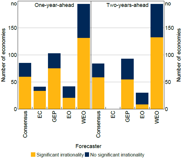
Notes: Test uses 5 per cent level of significance. The sample of two-years-ahead EC forecasts is small, so this series is not shown.
Sources: Authors' calculations; Consensus Economics; European Commission; IMF; OECD; World Bank.
Having found widespread irrationality, we now investigate the source of irrationality. First, we perform Wald tests of the null that the coefficients on past forecasts are zero, which we reject for most economies (Figure 10). As explained in Section 5.2.2, this indicates that the forecasters have a tendency to make forecasts that are too extreme or not extreme enough.
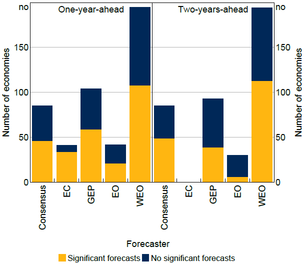
Notes: Test uses 5 per cent level of significance. The sample of two-years-ahead EC forecasts is small, so this series is not shown.
Sources: Authors' calculations; Consensus Economics; European Commission; IMF; OECD; World Bank.
Second, we perform Wald tests of the null that the coefficients on past errors are zero. Some forecasters, including the IMF, OECD and EC, only review their forecast performance every few years (Genberg et al 2014), so it is plausible that they would fail to make efficient use of any of the information contained in their recent errors. We reject the null that the coefficients on past errors are zero for a minority of economies (Figure 11). Since we conduct a separate hypothesis test at the 5 per cent level for each economy and forecaster, we would expect the Wald test to be rejected for 5 per cent of economies if the null hypothesis were true for all economies. These results provide tentative evidence that a failure to make use of the information in past errors is a source of irrationality for some forecasters for some economies, but suggest this issue is not too widespread.
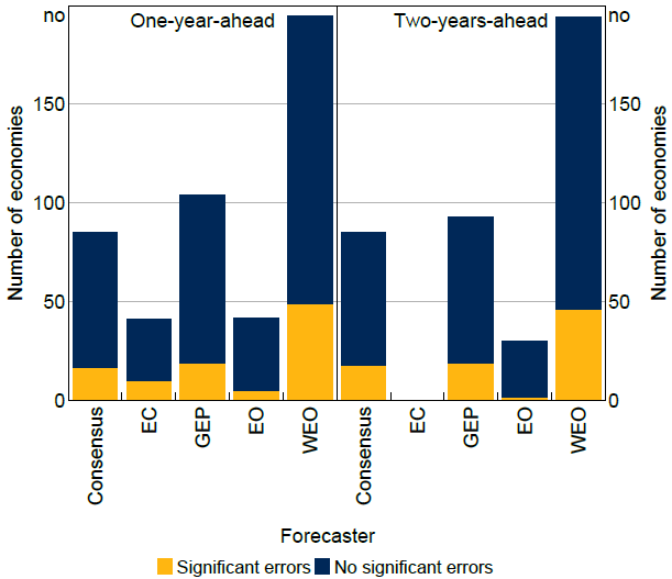
Notes: Test uses 5 per cent level of significance. The sample of two-years-ahead EC forecasts is small, so this series is not shown.
Sources: Authors' calculations; Consensus Economics; European Commission; IMF; OECD; World Bank.
5.3.2 Intercept and past forecasts specification
The Wald tests of the general specification suggest that failing to account for information in past errors is a relatively unimportant source of irrationality. For this reason, we consider a special case of the general specification where these past errors are removed:
We can view this regression through the lens of forecast revisions, which are changes in forecasts for a given target year from one vintage to the next. We rearrange the specification with forecasts only to obtain a specification with a forecast revision and a past forecast (Equation (7)).
The coefficient on the latest forecast revision tells us if the forecast revisions tend to be too large or too small. For example, if , it implies that if the forecaster revised up their forecast in the last period, , then the forecast error is likely to be positive, , which implies that the forecast error would be smaller if the upward forecast revision had been larger. Hence whenever we say that the latest forecast revision tends to be too small, indicating that the forecaster tends to underreact to the news received between t – 1 and t.[23]
We test rationality in Equation (7) by performing a Wald test of the null that all coefficients are zero (Figure 12). We reject rationality for many.
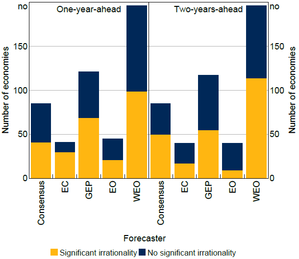
Note: Test uses 5 per cent level of significance.
Sources: Authors' calculations; Consensus Economics; European Commission; IMF; OECD; World Bank.
We know that this irrationality is not solely due to bias, because if we do a Wald test of the coefficient on the revision and on the past forecast, we reject the null for the majority of economies for all forecasters. To understand the role of revisions versus past forecasts, we do t-tests of each, noting that for some economies neither variable may be individually significant even though the two variables are jointly significant.
The t-tests of the coefficient on the past forecast show that this coefficient is insignificant in most economies (Figure 13). Where the t-tests are significant, the forecasts are typically too extreme. When the forecaster expects higher-than-average growth, they could improve accuracy by making a less optimistic forecast, and when the forecaster expects lower-than-average growth, they could improve accuracy by making a less pessimistic forecast. Halperin and Mazlish (2025) find, using regressions that pool across economies, that Consensus mean forecasts are too extreme. Their finding is consistent with our results, which show that Consensus mean forecasts are too extreme for a sizable minority of economies.
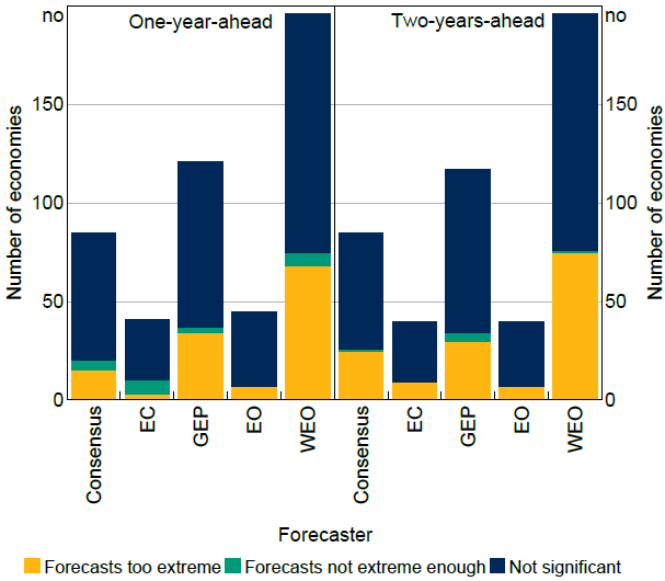
Note: Test uses 5 per cent level of significance.
Sources: Authors' calculations; Consensus Economics; European Commission; IMF; OECD; World Bank.
The t-tests show that the coefficient on revisions is significant in many economies (Figure 14). However, the direction of the inefficiency differs. In each international organisation, it is more common for revisions to be too large than for them to be too small. This is similar to the finding that individual private-sector forecasters make overly large forecast revisions (Bordalo et al 2020; Broer and Kohlhas 2024). For the average of Consensus forecasts, it is more common for revisions to be too small, consistent with previous evidence that the average of private-sector forecasts has overly small forecast revisions (Coibion and Gorodnichenko 2012, 2015). However, our finding contrasts with Halperin and Mazlish (2025), who find that average private-sector forecasts for real GDP have overly large revisions at horizons of two or more years.
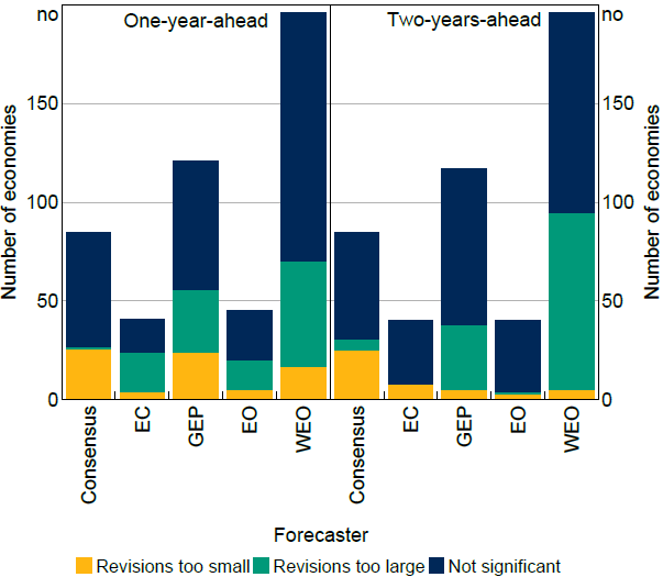
Note: Test uses 5 per cent level of significance.
Sources: Authors' calculations; Consensus Economics; European Commission; IMF; OECD; World Bank.
An alternative to regressing errors on forecasts (as we have just done) would be to regress forecast revisions on their own lags. Nordhaus (1987) shows that if forecasters incorporate all new information each time they update their forecasts, then the sequence of forecast revisions for a fixed target date will be serially uncorrelated. Such a sequence of forecast revisions is said to satisfy ‘weak efficiency’, which is a necessary condition for rationality. Hadzi-Vaskov et al (2021) find, using WEO real GDP growth forecasts, that the sequence of revisions for a given target year are negatively autocorrelated. This is consistent with our finding that WEO revisions are too large for a sizable minority of economies.
5.3.3 Intercept only specification
We also estimate a specification with the intercept alone. By doing this we are not claiming that the revision and past forecast are absent from the true model. As we saw earlier, the forecast revision and past forecast are jointly significant in most economies. Rather, we estimate this specification so that we can test for unconditional bias by performing a t-test of the intercept, as is standard in the literature. Although we could provide point estimates of unconditional bias in each economy using the previous specifications, we were not able to formally test if it was equal to zero.
For all forecasters, we find that there is no significant unconditional bias for most economies at the one-year or two-year horizon (Figure 15), though bias is more common at a two-year horizon for GEP and WEO. Where bias is present, it is almost always optimistic rather than pessimistic.
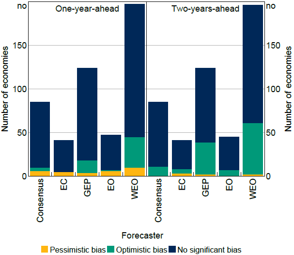
Note: Test uses 5 per cent level of significance.
Sources: Authors' calculations; Consensus Economics; European Commission; IMF; OECD; World Bank.
To summarise, we have shown that international organisations' growth forecasts fail rationality tests for the majority of economies. The reason for the rejection of this test differs by economy, but common reasons are that the forecasts are too extreme (Figure 13), revisions being too large (Figure 14), and optimistic bias (Figure 15).
Footnotes
That is, we assume that the part of the forecast errors not explained by the variables in our vector xt is covariance stationary. It is possible, for instance, that the forecast errors trend up over time, as long as this is explained by some variable in xt, so the errors do not trend up. [19]
Autocorrelation in the error would occur if, for instance, the error in the April 2020 forecast for growth in 2022 is correlated with the error in the April 2021 forecast for growth in 2023. It is plausible that these forecast errors could be serially correlated. For example, in 2020 the forecaster may forecast high growth in 2022, and 2021 they may forecast high growth in 2023. If an unexpected recession occurs that reduces growth in 2022 and 2023, the forecast errors for these two years will have the same sign. This could arise even if the forecaster is rational, because when the forecaster makes a forecast in April 2021 they have no way of knowing the error in the forecast they made in April 2020. One common response to autocorrelation in the error term is to model the dependence by including lags of the dependent variable as regressors. This solution is not appropriate here, as we want all the explanatory variables of a rationality regression to be known on the forecast date, and the lag of the dependent variable is a forecast error that is not known on the forecast date if the horizon is more than one period or the actuals are published with a lag. [20]
This is an exception to the way errors are usually computed in this paper, which is to use the latest vintage of the actuals (see Appendix A.2). [21]
This rearranged equation contains expectations of actual outcomes, forecasts and forecast errors. Hence, performing this rearrangement requires the additional assumption that these expectations exist and are constant. [22]
If we had regressed the forecast error on the past revision alone, then it would be unclear if the coefficient on the past revision reflected the forecaster's reaction to news (as we have claimed) or reflected that the level of the forecast was too high or low (as argued by Fuhrer (2018)). However, our regression should provide separate estimates of whether the forecaster responds efficiently to news (given by the coefficient on the revision, ) and whether the forecasts tend to be too extreme or not extreme enough (given by the coefficient of the second-latest forecast, ). [23]