RDP 2026-05: Real GDP Forecasts by International Organisations 6. Explanations for Rejection of Rationality

In Section 5, we conducted rationality tests for the forecasts from international organisations and Consensus by regressing forecast errors on an intercept, past forecasts for the target year and past forecast errors. Where the null hypothesis of the rationality test is false, then at least one of the following must be true:

• the forecaster does not satisfy forecast rationality;
• the forecaster must not have a squared error loss function; or
• the vector of explanatory variables, x_t must not be in the forecaster's information set.

If the null is false then this is likely because the forecaster does not satisfy forecast rationality or does not have squared error loss, rather than because the explanatory variables are absent from their information set. The reason is that the explanatory variables in our regressions are the forecaster's own forecast or the errors in their own forecasts, which are almost certainly known to the forecaster.

An extensive literature provides explanations for why different types of agents, such as consumers or firms, may make irrational forecasts. However, the explanations for irrationality at international organisations may be quite different, given that they make forecasts using different methods and face different incentives. In this section we consider two explanations that are based on specific features of international organisations:

1. International organisations make forecasts that are conditional on assumed future values of a variety of explanatory variables. Such forecasts violate forecast rationality under fairly general conditions (Section 6.1).
2. International organisations may report a ‘modal’ forecast, rather than a mean forecast (Section 6.2).

6.1 Conditioning assumptions

6.1.1 The rational expectations approach

Future growth, $y_{t+h}$, depends on the future values of a variety of explanatory variables, $x_{t+h}$, such as crude oil prices, exchange rates, nominal interest rates or government spending. As discussed in Section 5, if a forecaster has rational expectations and a squared error loss function, then their forecast will be a conditional expectation of growth given their information set.

By the law of iterated expectations, this rational forecast equals:

That is, the forecaster can make a rational forecast by:

1. Computing a conditional expectation of future growth given a value of the future explanatory variables, $E\left[y_{t+h}|x_{t+h},I_t\right]$, for each possible value of the explanatory variables; and then
2. Averaging this conditional expectation, $E\left[y_{t+h}|x_{t+h},I_t\right]$, over the various possible paths of the explanatory variables, weighted by the conditional probabilities of each possible value of the explanatory variables given the information set.

For example, one would compute the expected path for growth for each possible scenario for crude oil prices, and then compute a weighted average of those different paths for growth weighted by the likelihood of each crude oil price scenario.

6.1.2 The current approach at international organisations

International organisations make forecasts that are conditional on assumed future values of the explanatory variables.

In each WEO, the IMF publicly states its assumptions for exchange rates, oil prices, bond yields, monetary policy and fiscal policy. In addition, the IMF makes assumptions about other issues on an ad hoc basis. In the April 2021 WEO, for instance, the IMF made assumptions about COVID-19 vaccination and testing (IMF 2021).

The EC and OECD follow a similar practice of making assumptions about future explanatory variables such as exchange rates and then making growth forecasts conditional on those assumptions (Genberg et al 2014). Though central banks don't form part of our dataset, it's worth noting that they follow this practice as well (e.g. Kohler 2023). It's unclear what practices private-sector forecasters follow, as their forecasting processes are rarely as well documented publicly as those of international organisations.

6.1.3 Current practice typically differs from rational expectations

We will use the term ‘current practice’ forecast to refer to the conditional expectation of future growth $y_{t+h}$ conditional on an assumed future value of the explanatory variable $\widetilde{x_{t+h}}$.

Current practice will typically be inconsistent with rational expectations. This is true whether the assumed values of the explanatory variables are rational forecasts or not. We will consider each case in turn.

Case with rational forecasts for explanatory variable

First, suppose that the forecaster's assumed future value of the explanatory variable is a rational forecast for that variable, $\widetilde{x_{t+h}}=E\left[x_{t+h}|I_t\right]$. Then the current practice forecast will be:

Whether the current practice forecast of growth coincides with the rational forecast depends on two factors. Firstly, what is the relationship between future growth and the future explanatory variable? This relationship is described by the ‘response function’, $r\left(x_{t+h}\right)=E\left[y_{t+h}|x_{t+h},I_t\right]$. Secondly, what is the conditional distribution of the future explanatory variable given the information set? This is described by the conditional probability density function (pdf) $p\left(x_{t+h}|I_t\right)$.

The next theorem provides sufficient conditions for the current practice forecasts to be rational. For simplicity, the theorems and proofs consider a scalar explanatory variable. They condition on a fixed information set, omit that information set and the time subscripts from the notation, and denote $\mu \equiv E\left(x\right)$. We assume that $\mu$ and $E\left[r\left(x\right)\right]$ are finite.

Theorem 2. The rational forecast will equal the current practice forecast if:

1. the response function r is affine, that is, $r\left(x\right)=a+bx$ for constants a and b; or
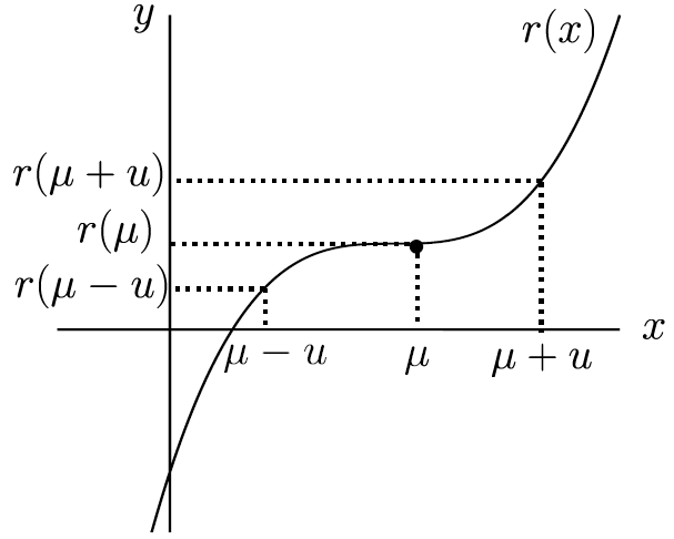
2. the response function r has 180 degree rotational symmetry about the point $\left(\mu ,r\left(\mu \right)\right)$, and the conditional pdf p is symmetric about its mean, $p\left(\mu -z\right)=p\left(\mu +z\right)$.

Proof. See Appendix C.

To give intuition for the theorem, the rational forecast of y considers the possibility that x could be above its mean and that x could be below its mean. Under the assumptions of this theorem, these two considerations have exactly offsetting effects, so the rational forecast coincides with the current practice forecast, which assumes that x will equal its mean. Consider case (b) where r satisfies the rotational symmetry assumption. As illustrated by Figure 16, if the explanatory variable is a distance u above its mean, the response function would change by $\left(r\left(\mu +u\right)-r\left(\mu \right)\right)$. If the explanatory variable were the same distance below its mean, the response function would change by $\left(r\left(\mu -u\right)-r\left(\mu \right)\right)$. The rotational symmetry assumption states that these two changes are the same in size and opposite in sign.

Since the future explanatory variable has a symmetric distribution about its mean, it is just as likely to be above its mean by u units as below its mean by the same amount. Hence, the rational forecast equals the current practice forecast.

If either of these symmetry conditions fail, then the current practice forecast may differ from the rational forecast, as we now show.

Theorem 3. Suppose the future explanatory variable has a non-degenerate distribution.

• If the response function r attains a strict global minimum (maximum) at the rational forecast for the explanatory variable, $\mu$, then the rational forecast will be strictly greater than (strictly less than) the current practice forecast.
• If the response function r is strictly convex (strictly concave), then the rational forecast will be strictly greater than (strictly less than) the current practice forecast.

Proof. See Appendix C.

To illustrate, consider the dependence of real GDP growth on rainfall, which may be important in low-income economies where agriculture is a large share of GDP. Typically, the kinds of agriculture undertaken in a given location are those that provide high yields when rainfall is typical for that location. For example, rice in areas with high rainfall and wheat in areas with lower rainfall. Hence it may be approximately correct to assume that real GDP growth in a low-income economy attains a strict global maximum at the average level of rainfall, or that growth is strictly concave in rainfall. If either of these assumptions is true, Theorem 3 implies that the rational forecast will be lower than the current practice forecast.

Case with irrational forecasts for explanatory variables

The preceding discussion assumed that the assumed future values of the explanatory variables are rational forecasts for those variables. This is likely to be approximately true when those assumptions are based on financial markets, as when crude oil price assumptions are taken from crude oil price futures. However, when assumptions are made in other ways they may be far from rational forecasts.

Assumptions about future fiscal policy will often differ greatly from rational forecasts. Where the IMF or EC are providing financing to an economy, they assume that the economy will fully implement any policies it agreed to as a condition of the financing (Genberg et al 2014). It is unlikely that expecting full compliance is a rational forecast, given that economies often comply only in part. For other economies, the IMF and EC approach:

assumes that policy changes will occur during the forecast period only if they have been legislated in advance or if there is substantial knowledge that suggests they will occur. Otherwise, policy is assumed to remain constant during the forecast period. (Genberg et al 2014, pp 35–36)

This is also unlikely to be a rational forecast, as it ignores the systematic tendency of governments of advanced economies to vary their fiscal policy to smooth out business cycle fluctuations.

6.2 Modal forecasts

6.2.1 Which forecasters make modal forecasts?

For a given conditional distribution of future growth, a forecaster could report the mean, the mode, the median, or some other summary statistic. Surveys of professional forecasters typically do not specify the type of point forecasts respondents should provide. For example, Elliott et al (2008) notes that the US Survey of Professional Forecasters does not specify the type of point forecasts that respondents should provide. Similarly, international organisations refer to their forecasts using vague terms such as ‘central forecast’.

It's likely that at least some international organisations see themselves as making modal forecasts. One piece of evidence is that some major central banks make modal forecasts.^[24] This suggests international organisations may do the same, given that they use similar forecasting models, are staffed by economists with similar training, and follow similar internal processes during forecasting rounds.

Some private-sector forecasters may also see themselves as making modal forecasts. This view was held, for instance, by JP Morgan (Davies 2017).

6.2.2 How would modal forecasts affect rationality tests?

Consider a forecaster who is able to compute the conditional distribution of growth given the information available on the forecast date.

• The forecaster could report the conditional expectation of growth, $y_{t+h|t}=E\left[y_{t+h}|I_t\right]$. In this case, their forecasts would satisfy rationality tests. That is, their forecast errors $v_{t+h|t}$ would be orthogonal to any vector of known variables x_t (see Equation (1)).
• If the conditional distribution is unimodal, the forecaster could instead report the conditional mode of growth, $y_{t+h|t}=\text{Mode}\left[y_{t+h}|I_t\right]$. If the conditional distribution is also symmetric, then the mode would coincide with the mean, and these forecasts would satisfy rationality tests. However, if the conditional distribution is asymmetric, the mode could differ from the mean, and the forecasts may not satisfy rationality tests.

Modal forecasts may fail rationality tests due to bias (as recognised in Kangur et al (2019)). However, modal forecasts may also fail rationality tests due to correlations of forecast errors with other explanatory variables (which has not been recognised previously). Biased forecasts will cause the rejection of rationality tests whenever the vector x_t includes a constant, because the bias would lead to the coefficient on that constant being non-zero. As shown in Bekaert and Popov (2019) and Burgess et al (2021), past growth outcomes have been negatively skewed in most economies. If the conditional distribution of future growth given the forecaster's information set is also negatively skewed, then the mode will often exceed the mean, in which case modal growth forecasts will have an optimistic bias.

Modal forecasts may result in correlations between forecast errors and other explanatory variables. For example, suppose that growth is a realisation from one of two non-overlapping distributions: a ‘crisis’ distribution centred on –5 per cent, or a ‘non-crisis’ distribution centred on 2 per cent. Let the probability of a crisis next year be low. Assume that the conditional mode remains the mode of the non-crisis distribution even if the crisis probability varies. The mean will then depend on both distributions, while the mode will depend only on the non-crisis distribution. Suppose some variable in x_t, such as the debt-to-GDP ratio, is positively correlated with the probability of a crisis next year. Then that conditional expectation of growth will be a decreasing function of that variable, while the conditional mode of growth will be unrelated to that variable. This implies that, if the forecaster makes a modal forecast, their resulting forecast errors will be negatively related with that variable, causing the failure of rationality tests.

6.2.3 Empirical evidence on whether making modal forecasts introduces bias

We have just argued that the practice of making modal forecasts could result in biased forecasts. We now show empirically that modal growth outcomes tend to exceed mean growth outcomes, which suggests that this bias might arise in practice, but the effect is small. We also raise a methodological limitation that affects both our method and the similar method of Burgess et al (2021). Due to this limitation, it remains possible that making modal forecasts contributes greatly to bias or not at all.

Conceptual overview of method

Suppose that for any given economy and forecast horizon, the conditional mode for a period t equals the sum of a constant $\mu$, the conditional mean $E\left[y_t|I_{t-h}\right]$, and a mean-zero error e_t.

The constant $\mu$ is the expected difference between conditional mode and mean. This parameter determines whether a hypothetical forecaster that knew the conditional distribution of future growth would make biased forecasts if they reported the conditional mode rather than the conditional mean. Our aim is to estimate this parameter, so our empirical strategy is focused on growth outcomes (which are relevant to the hypothetical forecaster) rather than on the growth forecasts of any particular organisation.

Ideally, we would compute the mean and mode of the conditional distribution of future growth for a sample of periods. Using this sample, we could estimate Equation (8), giving us an estimate of the amount of bias that modal forecasting causes for that economy, $\widehat{\mu }$. We could also test the hypothesis that modal forecasting does not introduce bias, $\mu =0$, against the alternative that it does.

Unfortunately, we do not observe the conditional distribution of growth given particular information sets. Rather, we observe a set of growth outcomes, which provides information about the unconditional distribution of growth. Hence, we need to use our model of conditional distributions (Equation (8)) to make a prediction about unconditional distributions. We do this by taking expectations of Equation (8) over possible information sets.^[25]

We then make the further assumption that the unconditional mode, Mode[y_t], equals the expectation of the conditional modes, $E\left[\text{Mode}\left[y_t|I_{t-h}\right]\right]$. This assumption is a limitation of the method, as discussed below. With this assumption:

Given a sample of growth outcomes, we would like to estimate the unconditional mode and the unconditional mean, as the difference between them would provide an estimate of $\mu$. A challenge is that an economy's growth may be a non-stationary process, so its mean and mode may vary over time. For example, some east Asian economies such as Japan experienced high ‘catch-up’ growth followed by more moderate growth. To allow for this, we assume that an economy's growth is the sum of a deterministic component, b_t, and a stationary stochastic component, z_t.

Substituting this into Equation (9), and recognising that deterministic components can be taken outside of the mode or expectation operator, we have:

Hence, to estimate how much making modal forecasts introduces bias, $\mu$, we compute the estimated mode of detrended growth less the sample mean of detrended growth. This is somewhat similar to Burgess et al (2021), who compare the sample mean of detrended growth to the sample median of detrended growth.

Implementation and results

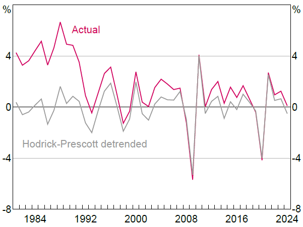
We use annual real GDP growth data from the WEO database for all economies whose time series has at least 40 observations. To estimate the stochastic component, we convert the growth rates into log levels, compute detrended log levels, and then compute growth rates of the detrended log levels. We detrend log levels using a two-sided Hodrick-Prescott filter (Hodrick and Prescott 1997), with the parameter value $\lambda =6.25$, following the recommendation for annual data given by Ravn and Uhlig (2002). Figure 17 compares actual growth rates, y_t, and our estimates of the stationary stochastic component, z_t, for Japan.

We estimate the mode of detrended growth using the half-sample mode estimator as implemented by the ‘modeest’ R package (Poncet 2019). This estimator assumes that the data are drawn from a continuous unimodal distribution, but does not require the assumption of any specific parametric distribution, and has the advantage of being insensitive to outliers (Bickel and Frühwirth 2006). We estimate the mean of detrended growth using the sample mean.

We find that 91 of 145 economies have an estimated mode above the sample mean. These differences are small in magnitude however. On average across all 145 economies, the estimated $\widehat{\mu }$ is 0.16 percentage points.

As a robustness check, we also compute the sample skewness of detrended growth for each economy:

Skewness is important because if the distribution of the detrended growth is unimodal, then its mode will typically exceed its mean when the distribution is negatively skewed. We find that 107 of 145 economies have negative sample skewness. This supports our finding that the unconditional mode exceeds the unconditional mean in most economies. Without this complementary evidence, one might have wondered if our results were driven by the specifics of our mode estimator.

Limitations

Our method assumes that the unconditional mode, Mode [y_t], equals the expectation of the conditional mode, $E\left[\text{Mode}\left[y_t|I_{t-h}\right]\right]$. This assumption holds exactly if the conditional mode does not vary with respect to variables in the information set. This is possible in principle. Returning to the example of a crisis introduced above, suppose that a crisis is very unlikely when the debt-to-GDP ratio (the variable entering the information set) is low and that a crisis is somewhat unlikely when the debt-to-GDP ratio is high. For both values of the debt-to-GDP ratio, the crisis will probably not occur, and the conditional mode of growth does not vary with respect to the variable in the information set.

It is more likely, however, that the conditional mode of growth does vary with respect to the information set. In this case, the assumption may or may not hold. We will illustrate this in the extreme case where the information sets fully determine growth. Suppose that there are three possible information sets: ‘pre-bust’, ‘ordinary’ and ‘pre-boom’, which guarantee that growth will be –2, 2 or 6 per cent respectively. First we consider the symmetric case, where ‘pre-bust’ and ‘pre-boom’ each occur with probability $\frac{1}{4}$ and ‘ordinary’ occurs with probability $\frac{1}{2}$. In this case, the assumption holds:

In practice, business cycles are likely to be asymmetric. Suppose that the probability of ‘pre-bust’ is $\frac{1}{4}$, of ‘ordinary’ is $\frac{3}{4}$ and of ‘pre-boom’ is 0. Then:

As this discussion illustrates, unconditional modes may differ from the expected conditional mode in the face of asymmetric business cycles, which is a situation we are interested in. Hence, one should be cautious about the results of our method (which suggest that modal forecasts may contribute slight optimistic bias), but also about any other effort to explain forecast bias using the unconditional distribution of growth. In particular, comparing the sample median and sample mean of growth as in Burgess, Langendorf, Ippolito and Pielke (2021) provides an unbiased estimate of the difference between the conditional median and conditional mean only if one assumes that $E\left[\text{Median}\left[y_t|I_{t-h}\right]\right]=\text{Median}\left[y_t\right]$, which is subject to an analogous critique.

Footnotes

The Bank of England refers to its forecasts as modal forecasts in its main public communications, such as its monetary policy report. Other central banks view themselves as making modal forecasts, but rarely use this term in public communications. Examples include Federal Open Markets Committee participants (Rudebusch 2008), the Federal Reserve Bank of New York (Alessi et al 2014) and the Reserve Bank of Australia (Debelle 2017). [24]

By the law of iterated expectations: $E\left[E\left[y_t|I_{t-h}\right]\right]=E\left[y_t\right]\forall t$. The error is zero on average across information sets by assumption. [25]