
RDP 2026-05: Real GDP Forecasts by International Organisations 4. Comparing Accuracy Across Forecasters
September 2026
- Download the Paper 2.9MB
4.1 Method
We compare the accuracy of different forecasters using Diebold-Mariano (DM) tests (Diebold 2015). We use WEO forecasts as our benchmark, and compare each other forecaster to the WEO. We perform this comparison separately for each economy and forecast horizon. WEO forecasts are available for a comprehensive set of economies, so using them as our benchmark maximises the number of economies for which we can perform comparisons.
In a DM test, the null hypothesis is that the pair of forecasters have equal forecast accuracy (i.e. equal expected loss), while the alternative is unequal forecast accuracy.
A ‘loss differential’ is the difference between the loss of the two forecasters, . The null hypothesis of the DM test is equivalent to stating that, in a regression of the loss differential on an intercept, the intercept is zero:
Under the assumption that the loss differential is covariance-stationary, the OLS estimator of the intercept is asymptotically normal. We perform the DM test by performing a two-sided t-test of the null that . We use heteroskedasticity and autocorrelation consistent (HAC) standard errors, as we want to allow for the possibility that the loss differentials are serially correlated.[10]
There are two further econometric complications. Firstly, our approach is only asymptotically valid, but the sample sizes in macroeconomic forecast evaluation are often modest. As Kiefer, Vogelsang and Bunzel (2000) explain, conducting t-tests with HAC standard errors in finite samples leads to rejecting null hypotheses more often than the chosen level of significance. The importance of this issue depends on the forecasters being compared. As shown in Table 1, our dataset includes many forecast vintages for the IMF, OECD and Consensus, but fewer for the EC and World Bank.
Secondly, the forecasts by international organisations and the private sector are often informed by models whose parameters are estimated on finite samples of input data. Even where the forecaster relies solely on judgement, they can be viewed as using an implicit mental model that is informed by the finite sample of input data. Diebold (2015) discusses alternative tests that aim to address this issue, and argues that using a DM test rather than the alternative tests is appropriate provided that the forecast errors are approximately covariance-stationary.
4.1.1 Timing issues
When computing loss differentials for an economy, we must ensure that the two forecasters record that economy's growth rates over the same period. Fortunately, WEO, EO, EC and Consensus all record each economy's annual growth rates over the same 12-month periods (see Appendix A). There are some economies where WEO and GEP record growth rates over different periods, so we do not compute loss differentials for these economies.[11] As an additional check, whenever both forecasters have data on actual outcomes, we check that the actual outcomes are the same.[12]
We also need to ensure that the loss differentials are computed with forecasts made around the same time. When comparing Consensus with an international organisation, we always compute loss differentials using forecasts made in the same month for the same target year. For example, if we wanted to compute a sequence of 14-month-ahead loss differentials, we'd compute one differential as ‘October 2020 WEO forecast for 2021’ with ‘October 2020 Consensus forecast for 2021’, and compute the next differential as ‘October 2021 WEO forecast for 2022’ with ‘October 2021 Consensus forecast for 2022’.
When comparing international organisations with each other, we compute loss differentials using forecasts made in the same or adjacent months for the same target year. For example, we could compute one differential as ‘October 2020 WEO forecast for 2021’ with ‘November 2020 EC forecast for 2021’, and compute the next differential as ‘October 2021 WEO forecast for 2022’ with ‘November 2021 EC forecast for 2022’. A limitation of this approach is that one forecaster will have an additional month of information relative to the other, giving them an unfair advantage in our comparisons of forecast accuracy. In practice, EC always has one more month of information than WEO, GEP has the same or less information than WEO, and the OECD sometimes has more information and sometimes less (see Table 2).[13]
| Publication month | EC | EO | GEP |
|---|---|---|---|
| 1 month before WEO | 0 | 18 | 9 |
| Same month as WEO | 0 | 2 | 14 |
| 1 month after WEO | 33 | 24 | 0 |
|
Sources: Authors' calculations; European Commission; OECD; World Bank. |
|||
4.2 Results
4.2.1 Diebold-Mariano tests for individual economies
We conduct a DM test for each economy and horizon. We report the p-value of each DM test. In addition, we report the ratio of the root mean square forecast error (RMSFE) of one forecaster to the RMSFE of the WEO.[14]
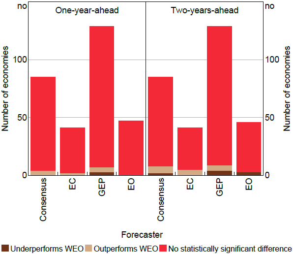
For the vast majority of economies, we find no statistically significant difference at a 5 per cent level in forecast accuracy (Figure 1). For the one-year horizon there are a handful of economies where Consensus and EC are found to outperform or underperform WEO, and at the two-year horizon there are a few economies where each forecaster outperforms or underperforms.
Note: Test uses 5 per cent level of significance.
Sources: Authors' calculations; Consensus Economics; European Commission; IMF; OECD; World Bank.
Since we perform DM tests separately for dozens of economies with a 5 per cent level of significance, even if the null hypothesis is true we would expect around 5 per cent of economies to show a significant result. This would be just two or three economies for EC, EO and Consensus, and zero or one economies for GEP. Hence, the handful of economies with statistically significant differences could be spurious. If one of the forecasters was genuinely better or worse in general, we would expect to see that forecaster outperform or underperform for many economies, but this is not the case. The results for each individual economy at a one-year-ahead horizon are available in Table B.1.
The lack of significant results could occur because there is genuinely no meaningful difference in performance, or because our sample sizes are too small to detect any performance differences. Our paper benefits from having access to more recent forecast vintages than earlier studies, increasing the power of our tests (see Section 2.1). Nevertheless, the sample sizes are modest. This is especially true for comparisons of GEP or EC, whose forecast vintages start in 2010 and 2011 respectively.
4.2.2 Cross-economy evidence
The hypothesis tests considered each economy in isolation. A natural question is whether one can better detect differences in forecast performance by drawing on the results for many different economies. Unfortunately, it is not straightforward to use the observed performance for different economies in a formal hypothesis test. The reason is that actual outcomes are correlated across economies (e.g. high growth in France tends to coincide with high growth in Germany), and forecasts tend to be correlated across economies too (e.g. if the IMF expects high growth in the United States it likely expects high growth in Mexico too). As such, the forecast errors for different economies do not provide independent sources of information.
Nevertheless, considering the results for many economies together provides suggestive evidence for differences in performance between forecasters. This suggests that, while tests of differences in forecast accuracy typically fail to reject the null at present (Section 4.2.1), future studies with longer sample periods may find differences more often.
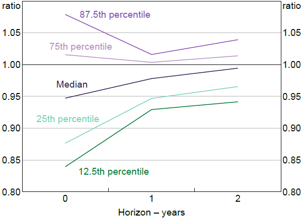
First we compare Consensus to WEO. For each horizon, we sort economies from the lowest ratio of Consensus RMSFE to WEO RMSFE to the highest. At zero or one-year horizon, roughly 75 per cent of economies had a lower Consensus RMSFE than WEO RMSFE (Figure 2). This provides suggestive evidence that Consensus mean forecasts are more accurate than WEO in general. Of course, absent a formal hypothesis test, we cannot say how likely it is that Consensus outperformed WEO by this much over the sample period simply by chance. If the Consensus mean is more accurate in general, it might reflect that combining forecasts of different forecasters tends to improve accuracy (e.g. Clements and Harvey 2009).
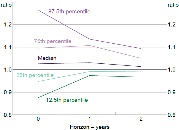
Second, we compare EO to WEO using the same exercise. At a one-year horizon, around 75 per cent of economies had a higher EO RMSFE than WEO RMSFE (Figure 3). This suggests WEO may be more accurate than EO in general. This cannot be attributed to differences in the timing with which each forecaster publishes their forecasts, because although the EO has a one month timing advantage in some vintages, it has a one month timing disadvantage in other vintages (Table 2).
We also compare both EC and GEP to WEO. These do not have a clear pattern in either direction. These point estimates are noisier, as the comparisons are based on a smaller set of vintages than EO or Consensus.
Sources: Authors' calculations; Consensus Economics; IMF.
Sources: Authors' calculations; IMF; OECD.
4.3 Decomposing differences in forecast performance
A loss differential measures the difference in accuracy of two forecasts for the same outcome. We show that in the case of squared error loss, a loss differential can be decomposed into two components: the accuracy of the average forecast and the disagreement between forecasters. This decomposition can be applied to any comparison of pairs of forecasters, as it is not specific to a particular variable (such as real GDP growth) or a particular type of forecaster (such as international organisations).
Theorem 1. Suppose the loss differential between a forecaster c and another forecaster b is computed with squared error loss:
Then the absolute loss differential can be written:
Proof. See Appendix B.1.
If we assume that the loss differential, the error in the average forecast, and the absolute difference in forecasts are all non-zero, we can take natural logs, giving:
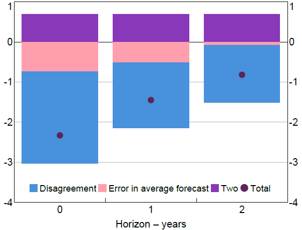
Before taking logs, we omit observations for which the absolute loss differential or either component is less than 0.01. We can use this decomposition to understand how the relative performance of a pair of forecasters for an economy depends on the forecast horizon. To do this, we compute sample means of the log absolute loss differentials across all forecast dates, and sample means of the components.[15] Figure 4 shows this decomposition for the Consensus and WEO forecasts for the United States. At longer horizons, the log absolute loss differential is less negative, which means the absolute loss differential is larger. Our decomposition shows that this occurs because longer horizons have both larger amounts of disagreement and larger errors in average forecasts.
The decompositions for individual economies are not too informative in our application. As discussed in Section 4.2.1, we find statistically significant differences in accuracy for only a few economies, possibly reflecting the modest sample sizes of forecasts. However, the decompositions for individual economies may be informative in future studies with larger sample sizes, including studies on other variables or types of forecaster.
Sources: Authors' calculations; Consensus Economics; IMF.
We also consider the results for many economies together, as this may reveal patterns that are hard to detect for individual economies. To do this, we perform the decomposition for each individual economy, and then summarise the results by estimating a panel regression (Equation (2)). The dependent variable is the log absolute loss differential for a particular economy i, forecast month t and horizon h. The explanatory variables are economy fixed effects and dummies for each horizon. We include a horizon dummy for each horizon h = 1,...,H, which means the base case is a horizon of h = 0 years.[16] The economy fixed effects are included because the magnitude of loss differentials is likely to differ across economies.[17]
We then perform two more panel regressions with the same explanatory variables, but where the dependent variable is a term from our decomposition (Equation (3)).
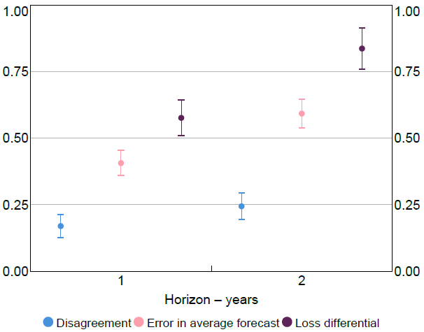
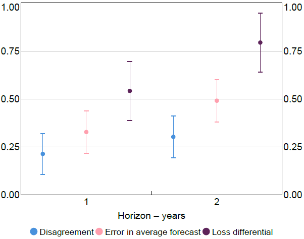
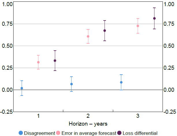
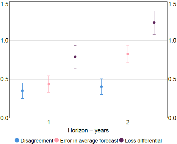
Figure 5 shows the estimated coefficients on the horizon dummies for the comparison of Consensus to WEO. Figures 6, 7 and 8 do the same for comparisons involving EC, GEP and EO respectively. Across all four pairs of forecasters, we find that, relative to the zero-year-ahead base case, the log absolute loss differentials are larger at a one-year horizon, and larger still at a two-year horizon. Our results show that, over the sample period, this occurred because the errors in the average forecast were larger at longer horizons, and to a lesser extent, because disagreement between the forecasters was larger at longer horizons. Whether this is true in the population is hard to assess.[18] It makes sense that the forecast errors and disagreement are both larger at longer horizons, since forecasters have less information at these horizons. In particular, the forecasts at a zero-year horizon typically benefit from having data for some quarters of the year.
Note: Whiskers show 95 per cent confidence intervals.
Sources: Authors' calculations; Consensus Economics; IMF.
Note: Whiskers show 95 per cent confidence intervals.
Sources: Authors' calculations; European Commission; IMF.
Note: Whiskers show 95 per cent confidence intervals.
Sources: Authors' calculations; IMF; World Bank.
Note: Whiskers show 95 per cent confidence intervals.
Sources: Authors' calculations; IMF; OECD.
Our results suggest that practitioners should be cautious when interpreting the size of loss differentials at different horizons: if the difference in squared errors becomes larger in magnitude at longer horizons, this does not necessarily indicate changes in the relative performance of the two forecasters, but rather could arise simply because both forecasters are less accurate at longer horizons.
Footnotes
We use the HAC estimator in the ‘sandwich’ package in R (Zeileis 2004) with the default options. [10]
GEP errors are computed using GEP forecasts and WEO actuals (see Appendix A.2). We abstain from computing GEP errors for any economy for which GEP and WEO record growth rates over different periods. Hence for these economies, we lack GEP errors, so we couldn't compute loss differentials even if we wanted to. [11]
Where we can compare actuals in this way, we remove the risk of accidentally comparing loss differentials whose actuals are recorded over different periods. Moreover, we avoid the risk of comparing loss differentials whose actuals differ for other reasons, such as differences in rounding conventions or data sources. [12]
The timing mismatches raise a subtle issue with forecast horizons. Each DM test is performed on a sequence of loss differentials with a specified forecast horizon, such as one-year ahead. Where a loss differential compares two forecasts published in the same month for the same target year, their forecast horizons are the same, and that loss differential can be viewed as having that horizon. However, where a loss differential compares two forecasts published in adjacent months for the same target year, their forecast horizons differ by one month. In this case the loss differential is labelled with the average of the horizons of the two forecasts being compared. [13]
This ratio is not the point estimate of the DM test statistic, which would be the mean square forecast error of one forecaster less than mean square forecast error of WEO. We prefer to report the ratio of RMSFEs as it is easier to compare across economies than differences in sample means, which are larger in magnitude for economies whose forecasts tend to be less accurate. [14]
In the empirical implementation, we omit observations for which the absolute loss differential, the absolute error in the average forecast, or the absolute difference in forecasts is less than 0.01 before taking logs. [15]
For example, the January 2021 WEO includes forecasts for growth in 2020 since actual outcomes are published with a lag. These forecasts would be considered to have a horizon of zero years, since their horizon in days rounds to zero years (see Section 3). [16]
For example, real GDP growth in an emerging market like India is typically higher and more volatile than in an advanced economy like Japan. Hence, the loss differentials are likely to be larger in India than in Japan. We include economy fixed effects, but assume the same coefficients on the horizon dummies for all economies. This implies that we allow for absolute loss differentials to be larger in some economies than others on average across all horizons, but we impose that the effect on absolute loss differentials of changing horizon is the same across all economies. [17]
The confidence intervals are computed with ‘classical’ standard errors. These confidence intervals may be too narrow or too wide if the error terms in the panel regressions, , are correlated across economies i or over time t. This is a strong assumption; actual outcomes and forecasts are correlated across economies (see Section 4.2.2), suggesting loss differentials may be correlated as well. Nevertheless, the pattern in the point estimates is qualitatively similar across the four pairs of forecasters, suggesting the pattern in the sample has not arisen purely by chance.
[18]