
RDP 2026-06: Perceived Monetary Policy Rules: Evidence from Professional Forecasters in Australia 4. Evolution of the RBA's perceived reaction function
October 2026
Figure 3 summarises the estimated coefficients from the baseline survey-based Taylor rule regressions over time. The top panels report the estimated inflation coefficient from the simple specification (left) and the inertial specification (right), while the bottom panels show the corresponding unemployment coefficients. Shaded areas denote 95% confidence intervals, clustered by forecaster and horizon. Unless otherwise stated, the estimates are constructed using rolling four-quarter trailing samples to smooth high-frequency variation.
In what follows, we adopt a largely narrative-based approach, highlighting economically meaningful movements in the estimated coefficients and interpreting them in light of contemporaneous data, policy actions, and central bank communication. An alternative would be a more systematic regression-based analysis; however, the relatively short sample and the time-varying nature of policy communication limit the scope for such an approach. Given our focus on how communication and actions shape perceptions — and the likelihood that the relevant communication channels and messages evolve over time — a narrative interpretation is both informative and appropriate.
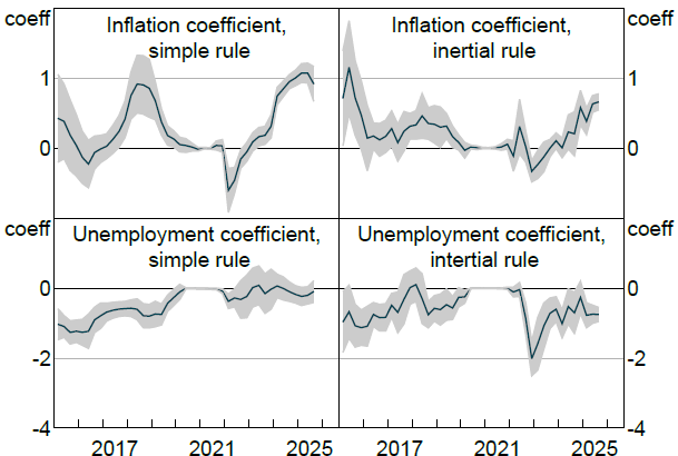
Note: Coefficients of perceived monetary policy rules estimated using 4-quarter rolling panel regressions on survey data from February 2015 to August 2025. Left panels show results from simple rules and the right from rules that allow for monetary policy inertia. Shaded areas indicate 95 per cent confidence intervals, based on standard errors clustered by forecaster and horizon.
4.1 Pre-pandemic dynamics
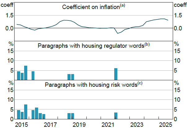
In the mid-2010s, forecasters inferred that the RBA placed only a modest weight on inflation in its perceived reaction function. This interpretation aligns with contemporaneous communication that foregrounded financial-stability considerations — particularly housing market risks — and signalled a reluctance to ease policy further despite persistently subdued inflation (Lowe 2016; Reserve Bank of Australia 2016). Simple text analysis supports this reading: references to housing risks and regulators in policy communications rose sharply in 2015–16, coinciding with the period in which the estimated inflation coefficient fell (Figure 4). While these correlations are descriptive rather than causal, the timing suggests that the financial-stability framing influenced how market participants mapped economic data into expected policy responses.
Notes:
(a) Coefficients of perceived monetary policy rules estimated using 4-quarter rolling panel regressions on survey data using simple rule.
(b) Paragraphs with both a housing and risk word, with no abating terms. Housing words include: dwelling prices, housing credit, housing market, housing conditions and household debt. Risk words include: downside risk, concern(s), and risk(s). Abating words include: eased, declining, decline(s), easing, fall(s) and abate.
(c) Paragraphs with both a housing and regulator word, with no abating terms. Housing and abating words as above. Regulator include regulator(s) and APRA.
Sources: Authors' calculation; RBA
Over the same period, the perceived response to unemployment gradually declined toward zero. This pattern is broadly consistent with a communication stance that elevated housing and financial-stability concerns, potentially reducing the salience of labour-market conditions in the perceived reaction function. However, the timing of movements in the unemployment coefficient is less tightly aligned with communication shifts than in the case of inflation.
Taken together, these findings suggest that RBA communication during the pre-pandemic period shaped perceptions of its reaction function. By emphasising financial-stability risks and signalling caution about further easing, the RBA appears to have dampened forecasters' perceptions of its responsiveness to inflation deviations from target, and (potentially) to a lesser extent to fluctuations in unemployment.
4.2 COVID and post-COVID dynamics: shifting emphasis back to inflation
A striking feature of the effective lower bound (ELB) period from 2020 to 2022 is the near-zero perceived responsiveness of the RBA to both inflation and unemployment. This pattern closely mirrors evidence for the U.S. Federal Reserve documented by Bauer et al (2024a) and recent evidence for Japan in Haba et al (2026). Interpretation of these estimates requires some care. When the policy rate is constrained by the lower bound, monetary policy may operate through forward guidance or other instruments that influence expectations and longer-term interest rates without necessarily generating variation in short-term interest-rate forecasts over the survey horizon. Our estimates therefore capture forecasters' perceptions of the responsiveness of the expected path of the cash rate to macroeconomic conditions, rather than the overall stance of policy. Accordingly, the near-zero coefficients suggest that forecasters viewed the expected cash-rate path over the forecast horizon as only weakly related to macroeconomic forecasts during this period, rather than policy overall being weakly related to conditions.
In the immediate post-pandemic period, the estimated coefficients in Figure 3 display a clear asymmetry. The perceived response to unemployment strengthens (in absolute terms) relatively quickly, particularly for the inertial rule, while the perceived response to inflation remains muted for an extended period. This pattern aligns closely with our language-based measures, which show a pronounced increase in references to “preserving labour market gains” across RBA policy announcement, speeches, and Minutes from early 2023 onward (Figure 5). It also aligns somewhat with the release of the (RBA Review Panel 2023), which reaffirmed the dual mandate nature of noting that “Equal consideration should be given to price stability and full employment in setting monetary policy”. Taken together, the coefficient estimates and the text evidence point to a phase in which markets inferred that policy was prioritising the recovery and durability of employment, while largely looking through temporary, supply-driven inflationary pressures—consistent with delayed policy lift-off and the tenor of RBA communication at the time.
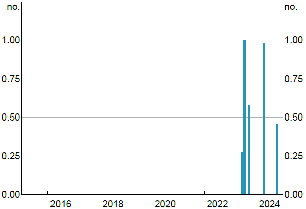
Note: Number of mentions of phrases related to preserving labour market gains in RBA policy meeting announcements, Minutes, Statement on Monetary Policy, and speeches. Quarterly totals per 10,000 words. Terms include ‘preserve the gains’, ‘preserve gains’, ‘preserve the employment’, ‘preserving the gains’, ‘preserve employment gains’.
Sources: Authors' calculation; RBA
A further salient feature of RBA communication during this period was the emphasis on sustained wage growth as a precondition for a durable return of inflation to target from late 2021.[4] To assess whether this framing shaped forecasters' perceptions, we augment the perceived reaction function to include a direct response to wage inflation, measured using forecasts of the WPI. Incorporating WPI leaves the estimated inflation and unemployment coefficients largely unchanged, indicating that our baseline results are not driven by omitted wage dynamics. However, the extension reveals that the perceived response to wage growth begins to rise in late 2021 before the inflation and unemployment coefficients increase, consistent with the view that markets interpreted wages as an early conditioning variable for policy normalisation (Figure 6).
As the tightening cycle progresses, the perceived inflation coefficient rises materially, signaling a reassessment of the Bank's willingness to respond forcefully to persistent inflation. By contrast, the unemployment coefficient exhibits no comparable and sustained rebound, remaining relatively subdued in the simple specification, with only a temporary increase in the inertial specification around 2022. Overall, the evidence points to a transition from an initial post-pandemic emphasis on labour market preservation toward a renewed focus on inflation, as policy actions accumulated and macroeconomic conditions evolved.
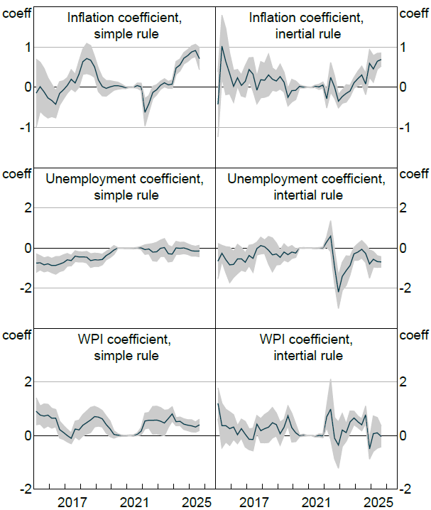
Note: Coefficients of perceived monetary policy rules estimated using 4-quarter rolling panel regressions with WPI. Left panels show results from simple rules and the right from rules that allow for monetary policy inertia. Shaded areas indicate 95 per cent confidence intervals, based on standard errors clustered by forecaster and horizon.
4.3 Why did the perceived inflation response rise only after lift-off?
A striking feature of the estimates in Figure 3 is that the perceived response to inflation remained subdued throughout 2021 and into 2022, despite large and persistent inflation surprises, and rose sharply only after the RBA began tightening policy in May 2022.[5] This pattern is particularly notable given that RBA communication became progressively more hawkish over this period, even if it did continue to highlight the importance of preserving labour market gains.
This disconnect is illustrated in Figure 7, which plots the perceived inflation coefficient alongside a text-based measure of policy tone: a Hawk–Dove index constructed separately for meeting minutes and post-meeting statements by Jones (2025).[6] The tone of RBA communication shifts decisively in a hawkish direction prior to lift-off, with the index rising markedly in late 2021 and early 2022. Yet over this same period, the estimated inflation coefficient remains low.
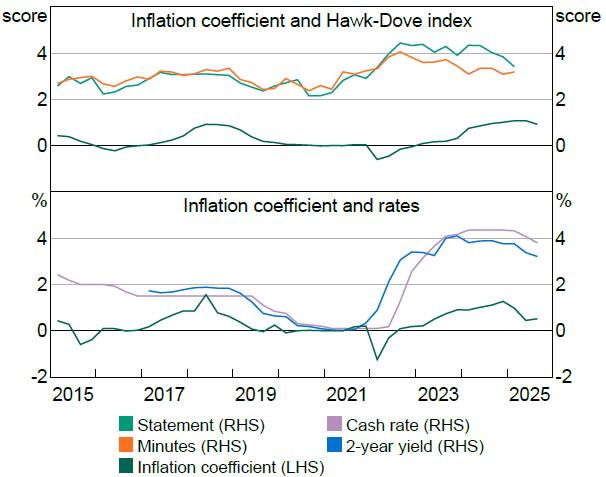
Note: Statement and Minutes series are quarter average Hawk-Dove indices from Jones (2025). Inflation coefficient are from simple monetary policy rules estimated using 4-quarter rolling panel regressions. Cash rate and 2-year yield are quarter averages.
Sources: Authors' calculation; Jones (2025)
Why was communication insufficient to induce an earlier reassessment of the perceived inflation response? Following Bauer et al (2024a), who document similar patterns for the United States and the euro area, we consider three potential explanations for the delayed increase in perceived policy responsiveness: (i) forecasters viewed the inflation surge as transitory; (ii) forecasters expected a persistent “lower-for-longer” policy framework; and (iii) forecasters primarily learned about the reaction function from realised policy actions under heightened uncertainty.
4.3.1 Transitory inflation views
One potential explanation is that market participants viewed the inflation surge of 2021 as largely transitory. Under this interpretation, forecasters would have expected inflationary pressures to fade without requiring a strong monetary policy response, leading them to anticipate little immediate adjustment in the RBA's reaction function.
To assess this hypothesis, we partition forecasters into two groups based on whether their inflation forecasts lie above or below the cross-sectional median. If forecasters who anticipated more persistent inflation also expected a stronger policy response, they should have projected an earlier and more pronounced lift-off from the effective lower bound.
In practice, however, the two groups forecast remarkably similar paths for the cash rate during and following lift-off (Figure 8). This similarity indicates that differences in beliefs about inflation persistence alone cannot account for why the perceived inflation response remained muted until after policy tightening had begun.
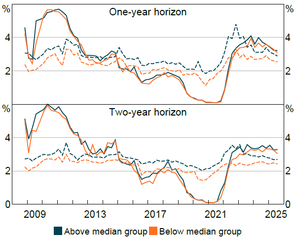
Note: Dashed lines are inflation forecasts, full lines are cash rate forecasts. Means within groups.
Sources: Authors' calculation; RBA
4.3.2 History-dependent or “lower-for-longer” expectations
A second possible explanation is that forecasters interpreted the RBA's strategy as history dependent. For example they may have expected the RBA to allow inflation to temporarily overshoot the target following a prolonged period below it, akin to an average-inflation or price-level target. Or alternatively, they may have taken perceived forward guidance and yield curve targeting as an implicit promise to keep rates low even if inflation rose. If this was the case, variation in inflation outcomes may have been unlikely to influence short-term policy rate expectations. However, they should still have had some impact on longer-term rate expectations.
This provides a simple empirical diagnostic to test whether such dynamics can explain the delayed pick-up in the inflation coefficient. If policy were perceived as strongly history dependent in this manner, inflation surprises should be associated with revisions to the expected medium- to long-run policy path, and so longer-term interest rates, even while near-term rates remained anchored. Figure 9 evaluates this prediction by plotting rolling correlations between inflation surprises (measured relative to Bloomberg median forecasts) and interest rates on Australian Government Securities at various maturities
The evidence provides little support for such a pattern. There is no economically meaningful increase in the sensitivity of longer-term rates to inflation surprises during this period; if anything, correlations at shorter maturities tend to rise earlier.[7] This is the case even if we focus on yields beyond the RBA's target yield for yield-curve control, which would appear to be a natural cut-off for the lower-for-longer dynamics to be most evident.
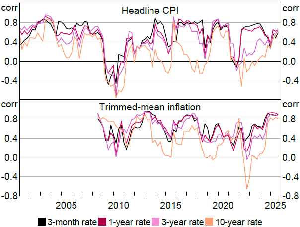
Note: Yield changes measured from previous close to close on day of CPI release. Inflation surprises are measured as gap between median Bloomberg forecast on day before the release, and the release. Headline CPI uses historical releases. Trimmed mean are most recent vintage pre 2012.
Sources: Authors' calculation; Bloomberg; RBA
4.3.3 Learning from monetary policy actions under uncertainty
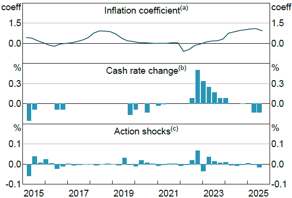
The third and most consistent explanation is that forecasters required concrete policy actions to update their beliefs about the RBA's reaction function. During 2021–22, uncertainty surrounding the near-term policy outlook was unusually elevated: communication emphasised labour market recovery and patience, while global inflation dynamics were shifting rapidly. As shown in Figure 10, the dispersion of one- and two-year-ahead cash rate expectations widened sharply as market participants attempted to infer both the timing and the pace of future tightening. Following the onset of rate increases in May 2022, and as tightening continued through 2023, this dispersion narrowed, suggesting that realised policy actions clarified the Bank's intentions, potentially alongside some increased certainty around the nature and persistence of economic shocks.
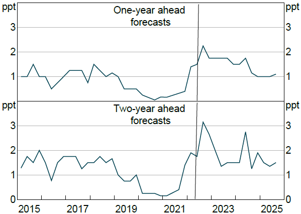
Note: Range of cash rate forecasts in the survey for each horizon. Solid line is May 2022 when cash rate hiking cycle began.
Sources: Authors' calculation; RBA
High-frequency evidence reinforces this interpretation. Figure 11 plots changes in the policy rate and high-frequency identified shocks monetary policy ‘Action’ shocks taken from Hambur and Haque (2024). The magnitude of policy surprises increased sharply following lift-off, consistent with substantial revisions in beliefs about the policy rule. Had market participants already internalised the RBA's intended strategy, post-announcement yield movements would have been more muted. Instead, the evidence suggests that forecasters learned about the renewed primacy of inflation control primarily from realised policy decisions.
Taken together, these results indicate that the re-anchoring of policy perceptions after 2022 was driven less by forward guidance and more by the sequence of actual rate increases. In periods of heightened uncertainty, communication alone proved insufficient; sustained policy actions provided the clearest signal of the RBA's true reaction function.
Notes:
(a) Coefficients of perceived monetary policy rules estimated using 4-quarter rolling panel regressions and simple rule.
(b) Change in cash rate. Quarter average.
(c) ‘Action shock’ from Hambur and Haque (2024). Quarter average.
Sources: Authors' calculation; Hambur and Haque (2024); RBA
4.4 Aiming for the stars
As discussed in Section 2, our baseline specification uses forecaster–time fixed effects to absorb forecaster-specific views about long-run “star” variables, including the neutral real rate, the NAIRU, and the inflation target (or long-run inflation). A natural question is how effectively these fixed effects capture long-run beliefs when recovering the perceived policy rule.[8] By relying on within-forecaster, cross-horizon variation, this approach deliberately abstracts from level differences across forecasters. While this helps isolate perceived policy slopes, it may also discard potentially informative cross-sectional variation if long-run beliefs themselves contain economically relevant information.
To assess this issue, we exploit the fact that the MES includes explicit questions on the NAIRU, long-run inflation, and the long-run equilibrium nominal interest rate (i.e. the nominal neutral rate) from 2024 on.[9] Figure 12 shows the dispersion of these expectations over time. We can see that there is notable and time-varying divergence, including in long-run inflation expectations, which reinforces the point that time-varying and heterogeneous expectations for star variables could be an important factor in estimation of perceived reaction functions.
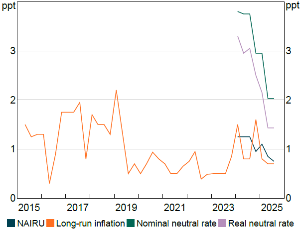
Note: Real neutral rate is nominal neutral rate less long-run inflation forecast.
Sources: Authors' calculation; RBA
Using these data, we re-estimate the model without forecaster fixed effects and instead directly incorporate forecaster-specific estimates of the star variables. We consider two variants. In the first, ‘Star model’, we include forecaster-level estimates of all three star variables. In the second, ‘Star model—constrained’, we impose a common inflation target of 2.5 per cent and replace only the neutral rate and NAIRU with forecaster-specific estimates. This comparison allows us to assess whether the observed dispersion in long-run inflation expectations reflects noise, or instead captures systematic differences in forecasters' broader views of the economy. The distinction is important for understanding how well inflation expectations are anchored.
Figure 13 summaries the results. First, the baseline and Star model estimates are very similar, both in levels and in their evolution over time. This finding suggests that the fixed-effects approach advocated by Bauer et al (2024a) and Bauer et al (2024b) provides a good approximation when direct measures of star variables are unavailable. Second, the Star model – constrained yields noticeably lower estimated inflation coefficients. Imposing a common long-run inflation expectation leads to a significant downward bias: forecasters with higher long-run inflation expectations — and therefore higher short-horizon inflation forecasts — are incorrectly treated as expecting larger inflation gaps. Because these forecasters do not, on average, expect correspondingly higher policy rates once differences in nominal neutral rates are taken into account, the estimated relationship between inflation gaps and expected interest rates is attenuated.
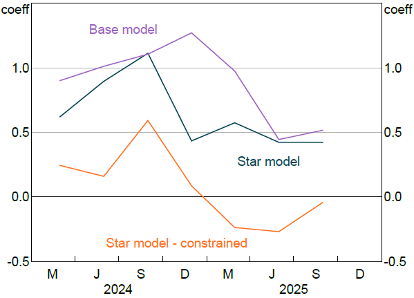
Note: Star model – constrained enforces long-run inflation coefficient of 2.5
Overall, the evidence indicates that variation in long-run inflation expectations is both economically meaningful and systematically related to forecasters' broader macroeconomic views. This suggests that monitoring the distribution of long-run inflation expectations — not just their average – can provide valuable information about how monetary policy is perceived and how expectations are anchored.
4.5 Sensitivity analysis
We assess the robustness of our results to a range of modeling choices. First, Figure 14 compares estimates from the inertial specification obtained using Arellano–Bond GMM with those from an OLS estimator with fixed effects. The resulting time profiles are similar, particularly for the inflation coefficient. The confidence bands largely overlap, and the key qualitative features, namely muted responsiveness in the mid-2010s and near-zero coefficients during the effective lower bound period, are preserved. One notable difference is that the inflation coefficient rises somewhat earlier under OLS, underscoring the importance of using an appropriate dynamic panel estimator when interpreting the timing of changes in perceived policy responsiveness. Differences are more pronounced for unemployment, with GMM yielding more negative estimates around 2022, consistent with it correcting the small-sample bias that arises in dynamic panels with lagged dependent variables.
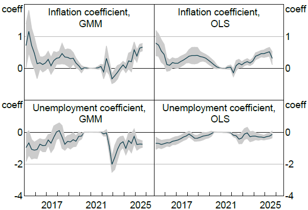
Note: Coefficients of perceived monetary policy rules estimated using 4-quarter rolling panel and inertial rules. GMM series apply Arellano–Bond GMM dynamic panel estimator. OLS series apply OLS. Shaded areas indicate 95 per cent confidence intervals, based on standard errors clustered by forecaster and horizon.
Sources: Authors' calculation; RBA
Second, Figure 15 reports quarter-by-quarter estimates rather than rolling-window averages. Although these series are naturally noisier, they convey the same message: perceived policy responsiveness to inflation is muted in the mid-2010s, close to zero during the effective lower bound period and rises materially thereafter once rates lift-off. The broad narrative is therefore unchanged, indicating that the headline results are not an artefact of the smoothing procedure.
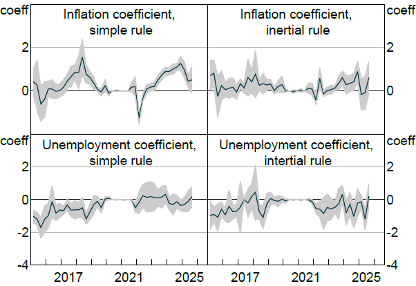
Note: Coefficients of perceived monetary policy rules estimated using quarter-by-quarter regressions on survey data. Left panels show results from simple rules and the right from rules that allow for monetary policy inertia. Shaded areas indicate 95 per cent confidence intervals, based on standard errors clustered by forecaster and horizon.
Sources: Authors' calculation; RBA
Finally, we examine the robustness of our maintained assumptions that policy coefficients and star variables are constant across horizons. Two considerations motivate this exercise. First, forecasters may perceive the RBA's reaction function itself to vary by horizon. For example, they may believe the RBA assigns less weight to inflation in the near term but more weight over longer horizons. Second, forecasters may have different degrees of confidence in their perceived policy rule across horizons, effectively implying horizon-specific error variances. This could arise if short-run policy decisions are viewed as subject to greater discretion or noise, while longer-horizon forecasts better reflect beliefs about the underlying reaction function.
To address these possibilities, we allow for horizon-specific weighting in the estimation, adopting an approach consistent with the latter interpretation. Under the inertial specification, a one-unit shock to the policy rate decays at a rate of approximately 0.7 per period. We use this implied decay to construct horizon-specific standard deviations and weight observations by their inverse, yielding a GLS-style estimator in which the error structure is disciplined by the model's dynamics.[10]
Figure 16 presents the resulting estimates. For both inflation and unemployment, the weighted and unweighted coefficients are nearly identical in both level and time profile. This similarity suggests that our assumptions of constant perceived reaction function parameters and star variables across horizons are reasonable and do not drive the main results.
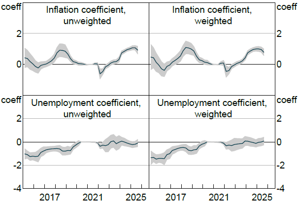
Note: Coefficients of perceived monetary policy rules estimated using 4-quarter rolling panel and simple policy rule. Unweighted series do not apply weights. Weighted series weight horizons based on the modeled shock decay rate. Shaded areas indicate 95 per cent confidence intervals, based on standard errors clustered by forecaster and horizon.
Sources: Authors' calculation; RBA
Footnotes
4 For example, the November 2021 policy announcement noted “The Board will not increase the cash rate until actual inflation is sustainably within the 2 to 3 per cent target range. This will require the labour market to be tight enough to generate wages growth that is materially higher than it is currently.” (Reserve Bank of Australia 2021)
5 The estimated inflation coefficient briefly turns negative during the transition to policy tightening. Such movements should be interpreted with caution and likely reflect the sharp change in expected conditions and central bank responses introducing noise into the estimation. For example, this same dynamic is less evident when the model is estimated period-by-period, suggesting that the pooling of periods across this volatile period is causing some estimation bias.
6 Methodologically, Jones (2025) construct the index using a supervised text-classification framework that guides a large language model with human-authored decision trees. Policy documents are scored on a five-point scale—dovish, leaning dovish, neutral, leaning hawkish, and hawkish—based on a balanced vocabulary capturing emphasis on inflation risks versus growth and labour market concerns, and then standardised for comparability across sources and over time. In this context, hawkish denotes a tighter policy bias, reflecting greater readiness to raise or maintain interest rates in response to inflation risks, while dovish indicates a greater emphasis on activity and employment risks.
7 A similar increase in the responsiveness of shorter-term rates has been documented in other advanced economies, including the United States, the euro area, Canada and the United Kingdom (Bauer et al 2024a; Xia and Zhu 2026).
8 More generally, the identification of latent macroeconomic “star” variables is known to be challenging and sensitive to modeling assumptions, even in structural state-space frameworks; see, for example, Buncic, Pagan and Robinson (2023).
9 Long-run inflation expectations are available for a longer period.
10 An alternative would be to weight observations using the empirical variance of cash rate forecast errors. However, such variances mechanically increase with the forecast horizon as additional shocks accumulate, and would introduce time-varying weights that complicate interpretation.