RDP 2026-02: Shifts in Australian Price-setting Behaviour around Large Shocks 4. Measuring Price Rigidity

Several ways of measuring price rigidity have been proposed in the literature. One is by simply looking at the share of prices that change in a month. However, this does not account for cases where prices may change multiple times in a month, which would abstract away from the richness of our high-frequency price data.^[9] Moreover, such measures do not account for how long a price has remained unchanged before adjusting – an important dimension of rigidity. Another approach is to look at the kurtosis of the distribution of price changes, which has been shown to provide a sufficient statistic for parameterising macro models with state-dependent pricing mechanisms (Alvarez et al 2016). However, kurtosis measures can be heavily affected by sample changes and noise.

Instead, we focus on measures of price duration – how many days since the price last changed. These overcome some of the above limitations and are well suited to our dataset. Moreover, they have a direct mapping to objects of interest in standard macroeconomic models of the business cycle, such as Calvo parameters.

4.1 Simple price duration measures

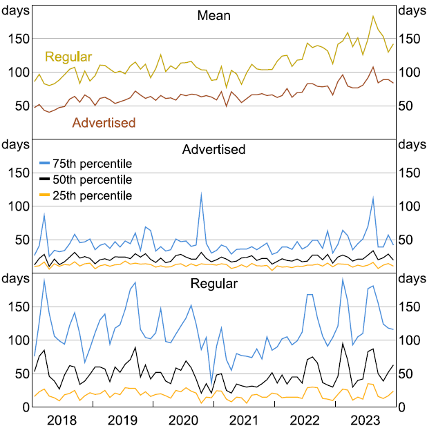
We start by showing the average number of days since an item last recorded a price change for all items that had a change in price. Following a period of relative stability through mid-2021, advertised and regular price durations rose as goods inflation rose, with longer intervals between changes on average (Figure 5, top panel). These results seem counterintuitive. However, they are largely explained by compositional effects. As inflation picked up, many prices in our dataset that had remained unchanged for extended periods – sometimes several years – began to adjust. The entry of these long-lived prices into the sample of changing prices increased the mean duration, even though firms were likely changing prices more frequently overall.

To see this, we can look at the distribution of price durations. The rise in average duration was concentrated in the upper tail of the distribution (e.g. the 75th percentile and above), while the median remained relatively stable (Figure 5, middle and bottom panels). The fact that long-stable prices began adjusting more often provides some initial evidence that price-setting frequency increased during the high-inflation period.

Note: Item-weighted.

Sources: ABS; Authors' calculations.

4.2 Survival analysis methodology

To explore this more formally we perform a survival analysis to estimate the probability that a price remains unchanged over time. This approach has several advantages. First, survival analysis incorporates the full set of price spells in the data, including prices that do not change.^[10] This makes it less sensitive to compositional changes in the sample driven by changes in very long-lived prices. Second, the regression-based framework allows us to formally test whether changes in rigidity over time are statistically significant. Third, survival models can control for firm-level heterogeneity and item censoring (where items enter or exit the sample mid-spell).

We use a parametric survival model with an exponential survival function, which assumes a constant hazard rate, that is, the probability of a price persisting is independent of information about how long it has been since that price last changed.^[11] This assumption aligns with the Calvo pricing model commonly used in DSGE frameworks, allowing us (through a simple conversion) to interpret the estimated survival rates of prices as Calvo probabilities.

The model is estimated by maximum likelihood over the full set of price spells, accounting for two key features of the data:^[12]

1. Firm fixed effects: these control for persistent differences in pricing behaviour across retailers, helping isolate within-firm changes over time and abstract from changes in the composition of firms in the sample.
2. Censoring: to address left censoring (e.g. unknown price history before an item enters the sample), we exclude the first observed spell for each item. The model also handles right censoring, where items exit the sample without a price change by incorporating this possibility into the likelihood function.

In our baseline specification, price survival probabilities are allowed to vary by the quarter or year in which a price spell begins.^[13] The estimation takes the following form:

where:

• S_ir (t|x_j) is the survival function giving a probability that the price of item i offered by retailer r remains unchanged for at least t days conditional on the year or quarter in which the price is observed x_j,
• ${\lambda }_r$ is a retailer-specific baseline hazard (rigidity) rate capturing firm fixed effects,
• x_j is a vector of indicator variables for the year or quarter associated with the end of a given price spell, and
• $\beta$ is a vector of coefficients on these time indicators, capturing period-specific survival rates across firms.

The survival function gives the probability that a price does not change up to a given point in time for each year or quarter in which underlying prices were observed. To make these results comparable to the Calvo parameter commonly used in macroeconomic models – which is expressed as the probability of a price remaining unchanged over one quarter – they are scaled to reflect the probability of prices remaining unchanged after 90 days (i.e. we set t = 90).^[14]

4.3 Survival analysis results

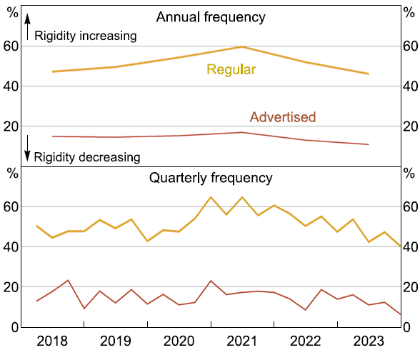
We estimate price rigidity separately for advertised and regular prices. As expected, regular prices are more rigid, reflecting the high prevalence of temporary discounting in advertised prices. On average, the probability that a regular price remains unchanged after one quarter is 51 per cent, compared with 14 per cent for advertised prices (Figure 6).^[15] These estimates are broadly consistent with empirical evidence from Sutton (2017). However, they imply greater price flexibility than standard macroeconomic models – an observation common in the international literature.^[16] For example, the RBA's DSGE model implies around 70 per cent of prices remain unchanged each quarter in the non-resource tradeables sector (which best aligns with our sample), and around 85 per cent on average across the broader economy.

We also find meaningful variation in rigidity over time. Regular prices became more rigid and less likely to change during the early pandemic period, with the probability of remaining unchanged rising by around 10 percentage points between 2019 and 2021. This was less evident for advertised prices, suggesting that firms were, in relative terms, relying more on discounting as a method for adjusting prices. This is consistent with heightened uncertainty evident during this period, which may have made firms relatively less willing to make more permanent price changes.^[17]

Notes: Item-weighted. Shading shows 95 per cent confidence intervals.

Sources: ABS; Authors' calculations.

From 2022 onward, as general retail goods inflation accelerated, both regular and advertised prices became significantly more flexible: by the end of the sample the share of advertised and regular prices remaining unchanged over a quarter was 25 and 7 per cent lower, respectively, than before the pandemic. This suggests that when faced with large inflationary shocks and rising input costs from 2022, firms started changing prices more regularly, including by making more permanent changes.^[18] This is consistent with international evidence that price rigidity tends to decline during high-inflation periods (see Cavallo et al (2024) and Gagliardone et al (2025)). It is also broadly in line with comparable overseas estimates, such as those documented using European CPI microdata in Gautier et al (2026).