
RDP 2026-02: Shifts in Australian Price-setting Behaviour around Large Shocks 6. How Shifts in Price Rigidity Affect Monetary Policy
May 2026
Changes in price-setting behaviour can have important implications for monetary policy. If price rigidity varies over time, then the transmission of monetary policy – and the trade-offs faced by policymakers, particularly during supply-side shocks – may also change.
In this section, we explore the implications of changes in price rigidity for monetary policy transmission, trade-offs and strategy. We conduct two exercises. First, we undertake a so-called optimal control exercise, calculating the policy paths that would have minimised (weighted) deviations of inflation and unemployment from target during the 2022–2023 high-inflation period under baseline model rigidity and under the lower rigidity observed in that period. Second, we examine how the optimal weights (those that minimise weighted deviations of inflation and unemployment) in a simple Taylor rule change as rigidity declines. This latter exercise is especially relevant in the context of supply-side shocks, where inflation and output move in opposite directions, creating a sharper policy trade-off. In contrast, demand-driven shocks typically move inflation and output in the same direction, making the implications of changing rigidity for those trade-offs less pronounced.
6.1 Transmission of monetary shocks under varying rigidity assumptions
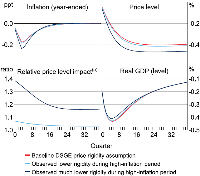
To motivate the analysis, we first simulate the impact of a 100 basis point monetary policy tightening shock under baseline and lower rigidity assumptions. The results show that when prices are more flexible, the disinflationary effect of a given rate increase is stronger (Figure 9). Crucially, this stronger inflation response is achieved without a larger decline in output. A steeper Phillips curve means that a given reduction in real activity translates into a larger fall in inflation. As a result, the trade-off between stabilising inflation and supporting real output is reduced.
Notes:
100 basis point positive shock in the cash rate.
(a) Ratio of the price level impact from the shock using alternative rigidity assumptions over impact using baseline rigidity.
Sources: ABS; Authors' calculations.
6.2 Optimal control exercises under varying price rigidity assumptions
We now examine how shifts in price rigidity affect monetary policy trade-offs and strategy. To do this, we implement an optimal control exercise using the DSGE model. Unlike a fixed policy rule approach (e.g. estimating a Taylor rule), optimal control calculates the path for the cash rate that minimises a standard policy loss function, given the shocks that hit the economy. This is a common method used by policymakers (e.g. Lowe and Ellis 1997; Adolfson et al 2011).
6.2.1 Methodology
For our analysis we assume that the loss function places equal weight on stabilising inflation, output (as a proxy for unemployment) and interest rate smoothing. Formally:
where:
- aj are the policy-relevant variables (inflation, output gap, and change in the nominal interest rate),
- are their respective ‘targets’ (2.5 per cent for inflation, 0 percentage points for both output gap and interest rate changes),[27]
- are the weights assigned to each variable,
- is the discount factor (set to 0.9996),
- the summation covers the period from March 2022 to December 2024.
Inflation and interest rate changes are each assigned a weight of 1. The output gap is weighted at 1/64, which equates a 1 percentage point deviation in inflation to a 1 percentage point unemployment gap, based on Okun's law. This implies equal weighting across inflation, unemployment, and interest rate volatility in the loss function.
We focus on unanticipated monetary policy shocks and do not compare the paths generated from this exercise with the actual policy response during the period, as this would not be a like-for-like comparison. Policymakers may have used a different loss function, and the model incorporates ex post information that was not available in real time. Instead, we compare paths under different rigidity assumptions to draw general lessons about how monetary policy should respond when price-setting behaviour changes, ceteris paribus.
6.2.2 Results
Figure 10 shows the policy paths from the exercise under baseline and lower rigidity assumptions. When prices are less rigid, the interest rate rises more aggressively in response to inflationary shocks. The cash rate peaks between 10 and 41 basis points higher than under baseline rigidity within the first year, resulting in substantially lower inflation.[28]
While output growth also declines slightly more than under the baseline, the trade-off is more favourable: the additional disinflation is achieved with only a modest additional fall in output. This reflects the steeper Phillips curve under lower rigidity, which allows inflation to be stabilised more effectively for a given change in real activity.
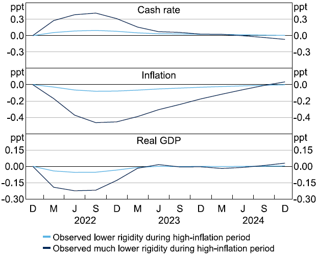
Notes: Cash rate path from optimal control exercise and associated inflation and real GDP outcomes under alternative assumptions about price rigidity. Results are shown relative to those obtained using the baseline price rigidity estimate embedded in the model. Inflation and real GDP growth are annualised growth rates.
Sources: ABS; Authors' calculations.
Overall, our findings suggest that when price-setting frequencies pick up – particularly during supply-side inflationary shocks – monetary policy can be tightened more aggressively to achieve faster disinflation with limited additional cost to output and unemployment. These results are consistent with those described in Karadi et al (2024), who conduct a similar exercise for the 2022-2023 US inflation surge using a model with state-dependent menu cost rigidities.
6.3 Optimal simple rules under different rigidity assumptions
While optimal control exercises provide a full policy path under a particular scenario, central banks often rely on simple policy rules – such as the Taylor rule – for communication, forecasting, and operational guidance. The Taylor rule prescribes a policy interest rate response given deviations in inflation and output from their targets (Taylor 1993). If price rigidity changes over time, and so the trade-off between inflation and unemployment changes, this could alter how aggressively policymakers want to respond to inflation and output fluctuations, and therefore the preferred weights in the rule.
To explore this, we assess how the coefficients in a standard Taylor rule that minimise a loss function vary under different assumptions about price rigidity. This helps quantify how monetary policy trade-offs evolve when firms adjust prices more flexibly, particularly during supply-side shocks.
6.3.1 Methodology
The Taylor rule specification embedded in the RBA's DSGE model takes the following form:
where:
- it is the nominal interest rate,
- it–1 is the lagged interest rate,
- r* is the neutral real interest rate,
- is the two-quarter-average inflation rate,
- is the inflation target,
- is the two-quarter-average GDP growth rate,
- and are the policy response coefficients to inflation and output, respectively,
- is the interest rate smoothing parameter,
- is a monetary policy shock.
To estimate how the values of and that minimise losses vary with price rigidity, we simulate the DSGE model under different Calvo parameters (as estimated in Section 4). For each rigidity setting, we solve for the Taylor rule coefficients that minimise the same policy loss function used in Section 6.2, subject to the model's structure and shock variances. In this sense, this exercise is thinking about what general rule would be optimal on average over all time under the different rigidities.[29]
6.3.2 Results
Under the baseline rigidity setting in the model, the loss-minimising weight on inflation is approximately 1.8 times the weight on output. When rigidity is lowered in line with observed changes during the post-pandemic inflation, this ratio increases to between 1.9 and 2.4 – a rise of 5 to 33 per cent.[30] These results are consistent with our earlier findings. When prices are more flexible, inflation responds more to changes in activity and the Phillips curve becomes steeper. As a result, placing greater emphasis on inflation in the policy rule is preferred. Our estimated ratios provide a simple metric for thinking about how the central bank's policy considerations might shift during large economic shocks that cause periods of elevated inflation and lower price rigidity.
Footnotes
More precisely the target for inflation is the average rate, which is closer to 2.6 per cent. [27]
A decline in price rigidity also implies a lower welfare cost of inflation, which could justify placing less weight on inflation in the policy loss function. We test a variant of the exercise where the inflation weight is reduced by 30 per cent, consistent with the decline in the social cost of inflation implied by lower rigidity in simple DSGE models (e.g. Blanchard and Galí 2010). While this adjustment brings the optimal policy path closer to the baseline, we caution against over-interpreting the result. The RBA's DSGE model is more complex than the stylised frameworks used to derive such adjustments, and the calibration of the weight change may not be directly transferable. [28]
One weakness of the approach is that the times that we face lower rigidities are exactly those times where the shocks hitting the economy are extreme. That said, the exercise still provides a general sense of the change in trade-offs. [29]
Note that both coefficients decline in absolute terms, particularly the output coefficient. This reflects the fact that, under lower rigidity, monetary policy has a stronger effect on real interest rates. Given this, demand shocks – which do not involve a trade-off between inflation and output – can be addressed with smaller interest rate adjustments. [30]