
RDP 2026-02: Shifts in Australian Price-setting Behaviour around Large Shocks 3. Data
May 2026
3.1 Data structure and treatment
The most commonly used types of price microdata in empirical research include survey data underlying consumer and producer price indices, scanner data sourced from point-of-sale transactions and prices collected from firms' websites (‘web-scraped’ prices). A discussion of the strengths and limitations of these types of prices in a research context can be found in Cavallo (2018). The present paper uses a web-scraped dataset from the Australian Bureau of Statistics (ABS) Business Longitudinal Analysis Data Environment (BLADE), which captures advertised prices for every item offered on up to 61 large Australian retailers' websites. Prices were collected every few days between 2016 and 2023, with the number of firms sampled increasing over time. The dataset becomes sufficiently large to be reliable from 2018 and in total has around 549 million price observations for 13 million unique items. While data collection occurred frequently across the dataset, the timing of collections was irregular.
The dataset covers a broad range of retail items, such as apparel, homewares, and electronic goods, which together represent around 25 per cent of the Australian consumer price index (CPI) basket.[3] Retailers and items are de-identified, though their industry classification is known. Two key attributes of sampled firms are that: (i) they derive substantial revenue from both online and brick-and-mortar stores; and (ii) they account for a large share of total turnover in their respective industry subdivisions – around 30 per cent across sampled firms in each quarter on average. These characteristics support two assumptions underpinning our analysis: that online advertised prices generally reflect in-store prices; and that price-setting behaviour observed in the sample can be generalised to the broader retail sector.[4]
Compared to some recent studies of price-setting behaviour – such as Auclert et al (2024) and Cavallo et al (2024) – our dataset includes a broader range of products, particularly discretionary and durable goods. These types of goods should exhibit slower-evolving pricing and longer item life cycles. In this sense, our data is more comparable to that used in Dedola et al (2023) and Blanco et al (2024a, 2024b, 2024c), which cover a wider set of products and services. This allows us to explore how retail firms with pricing that is typically less flexible respond to large economic shocks, and what implications this has for inflation.
The collection method used by the ABS for our dataset ensures that the full pricing life cycle of each item is captured – from the first day an item is offered for purchase to the day it is removed. This typically results in a downward-sloping price path for items over time. Measuring prices over the full life cycle of a product differs from conventional CPI price collection methods, where items are periodically substituted to control for quality changes within product categories. As a result, our dataset is likely to contain a higher share of price decreases than CPI data, making it unsuitable for calculating CPI-like average inflation rate measures but well-suited for measuring the breadth of offered prices across the products firms sell and for gauging shifts in price-setting behaviour.
There is ongoing debate about whether changes in advertised (sales-inclusive) or ‘regular’ (non-sale) prices are more relevant for characterising price rigidity. While some researchers argue that only regular price changes reflect firms' responses to macroeconomic shocks or cost pressures, others contend that both regular and sales price changes may shift in response to economic fundamentals and that what ultimately matters for inflation dynamics are the prices at which consumers transact.[5] This latter view aligns with the construction of the Australian CPI, which incorporates all advertised prices, including sales prices.
Rather than taking a firm position, we present rigidity results for both advertised and regular prices. While the ABS dataset contains both, regular prices are only available from 2020 onward. To avoid relying on a short sample and ensure consistent classification of sales prices across firms and over time, we develop an algorithm to identify active sales based on pricing patterns.[6] Specifically, we identify ‘V-shaped’ sales, where a price drops and returns to an equal or higher level within three months, and ‘clearance’ sales, where a price falls by at least 25 per cent and exits the dataset within a month. We use these imputed regular and sales price series in our analysis rather than the reported regular price data, though we find that the reported and imputed regular price data generally align well over time (Figures A3 and A4).
Importantly, while the levels of measured price rigidity in our dataset may differ substantially depending on whether sales prices are included, the changes in rigidity over time are similar across both price types. Given this, concerns about the inclusion of sales prices do not materially affect our conclusions about how shifts in price rigidity influence inflation dynamics and policy decision-making.
A further description of our data, cleaning methodology and sales algorithm is provided in Appendix A.
3.2 Summary statistics
To validate the data, we first provide some basic statistics and visualisations. Figure 2 shows the distribution of the log size of price changes in the data over the full sample period. Advertised prices exhibit symmetrical peaks around large changes such as ±25, ±30, and ±40 per cent, alongside a central concentration of smaller changes between –5 and +10 per cent (Figure 2, top panel). Disaggregating into regular and sales prices reveals that most regular price changes fall between –5 and +10 per cent (middle panel), while sales-related price changes are typically larger, clustering around common discount rates such as ‘25 per cent off’ (bottom panel).[7] The symmetry in sales price changes reflects items being discounted temporarily and subsequently returning to full price. As noted above, there is a relatively large tail of negative price changes, compared to what we might see if using CPI microdata. This reflects that the web-scraped prices capture the full life cycle from when items are first offered for purchase to when they are retired.
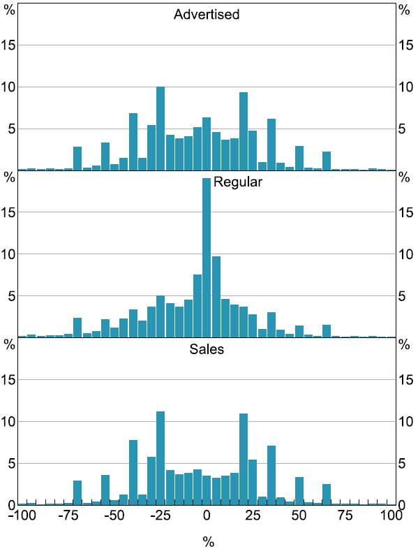
Notes: Item-weighted. x-axes are segmented in 5 percentage point intervals, where, for example, the zero bucket is changes between 0 and 5 per cent. Regular and sales prices are imputed using an algorithm that identifies sales patterns (see Appendix A).
Sources: ABS; Authors' calculations.
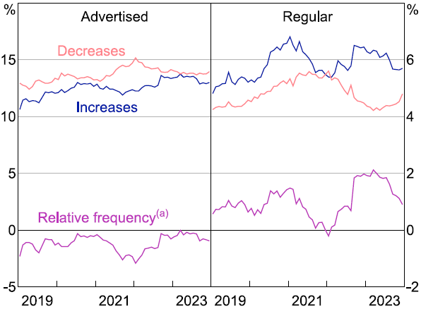
As a further validation, we look for evidence that the high-inflation period for goods is captured in our data. Given the nature of the data, rather than trying to recreate a CPI growth rate or focus on the size of price changes, we follow a number of other papers and look at the share of prices increasing and decreasing over each month (e.g. Bilyk et al 2024; Klein et al 2024). Specifically, we take the final price observation for each item in our data in each month and calculate the difference in the price compared to the end of the previous month. We then take the separate share of price increases and decreases out of all prices in each month, applying a 12-month trailing average to the resulting series to account for the highly seasonal nature of price setting. Subtracting decreases from increases provides a ‘relative frequency’ measure that can be used as a gauge for inflationary pressure. This approach abstracts from issues around life cycle pricing, as well as intra-month variation that is less relevant for observing the trend inflationary impulse.
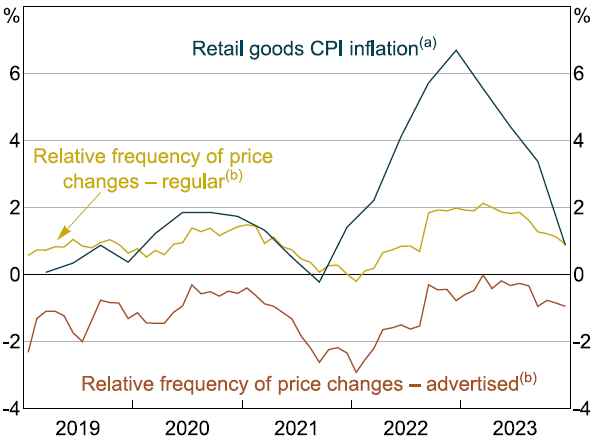
We find that the share of price increases rose notably over 2022 and 2023, while the share of price decreases declined (Figure 3).[8] This means that the relative frequency of price increases rose substantially, in line with the increase in retail goods price inflation (Figure 4). More generally, this metric has a close association with retail goods price inflation, picking up slightly in 2020, before declining in 2021 alongside inflation. These results suggest that the dataset does effectively capture the inflationary impulse seen in the official Australian CPI in 2022 and 2023.
Notes:
12-month trailing averages. All series are averaged across firms using CPI weights.
(a) Relative frequency is calculated as the percentage point share of all end-of-month item prices that constitute an increase compared to the previous month less the share that constitute a decrease.
Sources: ABS; Authors' calculations.
Notes:
(a) Year-ended growth in the ABS CPI goods component excluding items not in web-scraped dataset: food & non-alcoholic beverages, tobacco, new dwellings, motor vehicles and automotive fuel.
(b) Relative frequency is calculated as the percentage point share of all end-of-month prices that constitute an increase compared to the previous month less the share that constitute a decrease. Shares of increases and decreases are calculated as 12-month trailing averages. Averaged across firms in the web-scraped dataset using CPI weights.
Sources: ABS; Authors' calculations.
Footnotes
Items in the goods component of the CPI that are notably absent from the web-scraped dataset include food & non-alcoholic beverages, tobacco, new dwellings, motor vehicles and automotive fuel. [3]
These assumptions are standard in the web-scraped prices microdata literature, as well as in statistical agencies that collect online prices as a part of compiling official price indices. For example, see ‘Collecting prices for the CPI’ in ABS (2018). A further discussion of principles for selecting retail firms for web-scraping-based research can be found in Cavallo and Rigobon (2016). [4]
For contrasting views on the relevance of sales pricing to inflation dynamics and monetary policy analysis, see Guimaraes and Sheedy (2011) and Kryvtsov and Vincent (2021). [5]
This builds on the approach described in Gautier et al (2024). [6]
See Appendix B for figures showing how the distribution of the size of price changes has evolved over time. [7]
In general, there tend to be more price decreases than increases for advertised retail prices, and more increases than decreases for regular retail prices. This reflects that advertised prices include clearance sales while these are excluded from regular prices. [8]