
RDP 2026-02: Shifts in Australian Price-setting Behaviour around Large Shocks 5. How Shifts in Price Rigidity Affect Inflation Dynamics
May 2026
Having established in Section 4 that firms' price rigidity changed materially over the pandemic period and immediately after, we now assess whether these changes had meaningful implications for inflation dynamics. Specifically, we ask: if price rigidity declined between 2019 – our proxy for ‘normal times’ – and 2023 in line with our empirical evidence, how would this change have altered the transmission of shocks to inflation?
There are several ways to explore this question. One approach would be to build a new macroeconomic model calibrated to our microdata estimates. Another would be to incorporate our results into the RBA's existing benchmark DSGE model, which is used for policy analysis.[19] We adopt the latter approach, as it allows us to assess the implications of changing price rigidity within a framework familiar to policymakers. This helps bridge the gap between micro-level evidence and benchmark policy tools. Our exercise is similar in spirit to Gelain and Lopez (2024), who adapt the Federal Reserve's linear model frameworks to better capture inflation dynamics around the pandemic.
We focus on variation in the Calvo parameter – the probability that a firm does not adjust its price in a given period – which we estimated in Section 4 using survival analysis. Because the level of our estimated Calvo parameters differs from that used in the baseline DSGE model, we adjust the slope of the Phillips curve using the change in rigidity between 2019 and the peak of the inflation surge in 2023.[20] This embeds an assumption that ‘normal’ price rigidity in our data is best represented by the observed rigidity probability immediately prior to the start of the COVID-19 pandemic, and that the change in rigidity was similar across all goods and services in the CPI. We think this is broadly reasonable given the extended period of price stability prior to 2020. An alternative approach would be to test the effect of the shift in rigidity from its highest point in 2021 (immediately prior to the inflation surge) to its lowest point in the data during the surge in 2023. However, this would be less in line with the intent of comparing price rigidity at the peak of an inflationary episode to the normal rigidity embedded in our benchmark policy model.
5.1 Adjusting the slope of the Phillips curve
The RBA's DSGE model uses a Rotemberg-type price adjustment mechanism. To incorporate our Calvo-based rigidity estimates, we exploit the well-known equivalence between Rotemberg and Calvo pricing under a first-order approximation around the zero-inflation steady state.[21] This allows us to adjust the Phillips curve slope in the model using our estimated Calvo parameters. Specifically, the Phillips curve in the model can be expressed as:
where:
- is inflation,
- MCt is marginal costs,
- is a cost-push shock,
- is the slope of the Phillips curve, which is defined as:
Here, is the discount factor, is the degree of price indexation and is the Calvo parameter (the share of prices that remain unchanged in each period). Given the direct estimates of in the RBA's model and the parameters and , we can back out . We can then adjust using our microdata estimates to create an alternate Phillips curve slope .[22]
One natural question is how to map our estimated Calvo parameters into the model, given that there are levels differences between the estimated slopes in our empirical data and those embedded in the various sectors of the DSGE model. We test two approaches: one based on the absolute change in our estimate of rigidity (percentage points), and another based on the proportional change (per cent). These serve as lower and upper bounds for our analysis (Table 1).
| Advertised prices | Regular prices | |
|---|---|---|
| 2019 | 14.6 | 49.5 |
| 2023 | 10.9 | 46.1 |
| Lower bound difference (ppt) | −3.7 | −3.4 |
| Upper bound difference (%) | −25.3 | −6.9 |
| Sources: ABS; Authors' calculations. | ||
Rather than having a single Phillips curve, the DSGE model includes separate Phillips curves for each of five sectors: resources, tradeables, non-tradeables, imports and housing. We uniformly apply the observed variations in price rigidity between 2019 and 2023 to the slope of each curve; that is, we treat the observed shift in retail price rigidity as representative of a shift in economy-wide rigidity. Although this may seem a somewhat strong assumption, it is not obvious a priori whether other sectors would have experienced larger or smaller shifts. For example, applying the adjustment only to the tradeables sector would imply no changes in rigidity elsewhere in the economy, which is at least as strong an assumption as distributing the observed shift evenly across sectors.[23] While this choice affects the precise magnitudes of our quantitative results, it does not alter their qualitative implications.
5.2 Illustrating the role of price rigidity in the DSGE framework
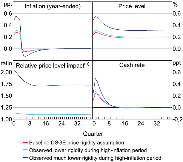
To illustrate the impact of price rigidity on inflation dynamics, we simulate a 1 per cent increase in the cost of foreign imports (i.e. a cost-push shock) in the DSGE model, using our estimated range of Calvo parameters for regular prices. We find that lower price rigidity leads to a stronger and faster inflation response. Specifically, the initial pass-through of the shock to year-ended inflation is higher by between 0.03 and 0.28 percentage points (Figure 7). The long-run impact on the price level also increases, rising from around 0.2 per cent under baseline rigidity to as much as 0.32 per cent under lower rigidity – an increase of nearly 75 per cent.[24]
Notes:
100 basis point positive shock in the price of foreign imports.
(a) Ratio of the price level impact from the shock using alternative rigidity assumption over impact using baseline rigidity.
Sources: ABS; Authors' calculations.
Given the DSGE model's Taylor rule, which includes inflation and a measure of real activity, this larger inflation response translates into a more aggressive policy interest rate path. The cash rate rises by between 3 and 25 basis points more in the first year compared to the baseline. Results are similar – but the cash rate increase is somewhat larger – when using the range of Calvo parameters estimated for advertised prices, which include temporary discounts and tend to be more flexible (Figure D1).
5.3 Forecasting inflation with time-varying price rigidity
The previous subsection illustrated how changes in price rigidity affect the transmission of a single shock. To assess the practical relevance of these changes, we now ask: if price rigidity declined between 2019 and 2023 as our estimates suggest, how much would this have affected model-based inflation forecasts during the post-pandemic surge?
To answer this, we conduct a scenario forecasting exercise using the DSGE model. We treat our microdata-based estimates of shifts in price rigidity as true and adjust the slope of the Phillips curve accordingly. We then use the model to recover the set of shocks that must have hit the economy to generate observed outcomes. Finally, we simulate the model forward from the start of 2022 using these estimated shocks but revert the Phillips curve slope to its baseline value. Comparing the resulting inflation forecasts to actual outcomes allows us to isolate the impact of misspecified price rigidity in the simulation. This approach is similar to that of De Fiore et al (2023), who use it to evaluate alternative monetary policy frameworks during the post-pandemic inflation period.[25] The exercise can be thought of as asking: how wrong would forecasters who only use the DSGE model have been if they had known all the shocks that were going to hit the economy, but didn't account for the fact that price rigidity had changed?
The DSGE model can be represented in its vector autoregression (VAR) form:
where:
- Yt is the vector of endogenous variables,
- is a matrix linking past values to current outcomes based on the model parameters,
- are structural economic shocks,
- is a matrix capturing the transmission of shocks based on the model parameters.
Changing the Phillips curve slope (via ) alters both and . Using our lower rigidity estimates, we denote the adjusted matrices as and , and the recovered shocks as . The model then becomes:
We take this set of equations to be the true structure of the economy, and so are the true structural shocks that were hitting the economy during the period, given the observed data.
With these true shocks in hand, we can then revert to the original model structure from 2022 onwards and calculate what forecasters might have expected inflation to be if they knew the shocks hitting the economy but had the wrong model structure and rigidity. The counterfactual conditions would be:
The difference between observed and counterfactual outcomes, , gives an estimate of the forecast error attributable to misspecified price rigidity.[26]
5.3.1 Results
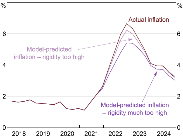
Figure 8 shows actual year-ended headline inflation alongside model-predicted inflation using the upper and lower bounds of our estimated rigidity decline. Even assuming perfect knowledge of the shocks, failing to account for the decline in price rigidity would have led the DSGE model to under-predict inflation by between 0.42 and 1.24 percentage points one year ahead. The peak of inflation would also appear slightly more persistent and delayed. The magnitude of these effects are broadly in line with findings in Gautier et al (2026), who argue that failing to account for changes in price-setting frequency in Europe during the post-pandemic high-inflation period would have led to inflation predictions being 1 percentage point lower.
These findings suggest that ignoring time variation in price rigidity – particularly during periods of large cost shocks – can lead to significant forecast errors. While our analysis is based on a DSGE framework, the implications are broader. Many forecasting models, including single-equation Phillips curves commonly used in public and private sector institutions, assume a fixed Phillips curve slope. Our results highlight the importance of allowing for time-varying price-setting frequencies when inflation dynamics are shifting rapidly and demonstrate that this was critically important during the recent inflationary episode.
As a supplementary exercise, we also tested whether varying the assumed degree of price rigidity affects the model's decomposition of inflation into supply and demand shocks. The results suggest minimal sensitivity to this assumption. See Appendix E for details.
Note: Actual inflation rate versus predicted path of inflation if price rigidity in the model was overestimated.
Sources: ABS; Authors' calculations.
Footnotes
This model is described in detail in Gibbs, Hambur and Nodari (2021). [19]
A formal Chi-squared test of estimated survival analysis coefficients showed that coefficients in each year after 2019 were statistically different from the coefficient in 2019. [20]
See proof and discussion in Rotemberg (1987) and Roberts (1995). [21]
For this analysis, we abstract from the price indexation term and assume it remains unchanged. [22]
That said, we acknowledge that some prices, such as administered prices that are indexed and updated on a set schedule, are unlikely to have had changes in their price-setting frequency in the high-inflation period. [23]
We also test the impact of a positive 1 per cent domestic consumption (demand) shock on the price level under alternative price rigidities; in general, the results are similar to those following the cost-push shock, though of somewhat smaller magnitude. For example, accounting for the decline in price rigidity with a consumption shock results in a price level estimate around 2 to 20 per cent higher in the long run. [24]
It is also somewhat similar to the decomposition in Lane (2024), where European inflation outcomes are decomposed into those reflecting incorrect assumptions about exogenous variables like energy prices, and those that cannot be explained by incorrect assumptions. [25]
One limitation of this approach is that the recovered shocks prior to 2022 are based on lower rigidity assumptions, whereas our results in Section 5 suggest that rigidity may have been higher during the early pandemic period. This could introduce minor bias due to autoregressive shock dynamics, but we expect the impact to be second order. [26]