
RDP 2026-02: Shifts in Australian Price-setting Behaviour around Large Shocks Appendix A: Data, Cleaning and Sales Algorithm
May 2026
A.1 Data description
A.1.1 Data collection
The raw data consists of prices for retail goods listed on the websites of major Australian retailers. These were collected by the Australian Bureau of Statistics (ABS) every few days between the start of 2016 and end of 2023. In general, the collection process involved taking the price of every item listed on a given retailer's website. The ABS performed some additional cleaning to reduce the likelihood that price collections were made for duplicates of the same item; however, in some instances it is possible that very similar items are recorded separately.[31]
Price collection dates vary by firm, and the frequency of price collections for a given firm may be irregular. For example, all prices for the items of a given firm might be collected on one date, then two days later, then four days later, then three days later, etc. The median frequency of price collections per item across firms is around six per month; this varies over time but generally increases over the sample (Figure A1).[32] Because of this, our main analysis of price rigidity uses a survival analysis method that accounts for bias from the irregular timing and frequency of price collections.
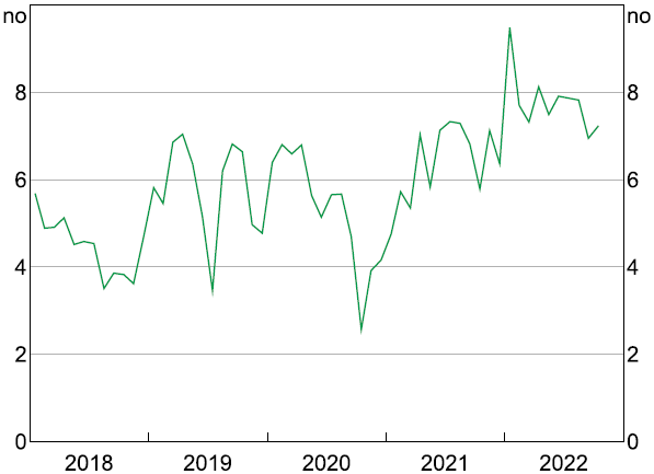
Sources: ABS; Authors' calculations.
A.1.2 Data fields
Data fields available for each retailer include a unique item number that is consistent across collection dates, the date of each price observation and up to three types of prices: ‘advertised’ prices, which are the current retail price of the item offered to consumers on that date (this may or may not be a discounted price); ‘regular’ prices, which are the undiscounted price of the item; and ‘sales’ prices, which are the price of the item if a sales event is active (Table A1). Advertised prices are available from the start of the dataset, while regular and sales prices are only available from 2020. The recording of regular and sales prices in the raw data reflects the classification of these price types by the retailers themselves as per their website. This means that there may be inconsistency in how sales activity is recorded across firms. For this reason, we standardise the definition of regular and sales prices across firms using the sales algorithm described in Section A.3.
| Retailer code | Retailer group | Item code | Date | Advertised price | Regular price | Sale price |
|---|---|---|---|---|---|---|
| 5 | clothing | 1 | 01/01/2020 | 20 | ||
| 5 | clothing | 1 | 03/01/2020 | 15 | ||
| 5 | clothing | 1 | 06/01/2020 | 15 | 20 | 15 |
| 5 | clothing | 2 | 01/01/2020 | 10 | ||
| 5 | clothing | 2 | 03/01/2020 | 12 | ||
| 5 | clothing | 2 | 06/01/2020 | 12 |
A.1.3 Firm and product types
The presence and total number of firms captured in the dataset varies over time, with the number of firms being too small to provide comfort about statistical validity of the sample prior to 2018. Between 2018 and 2023, the average number of firms present in each month is 53 and the total number of unique firms is 61 (Figure A2). Each firm in the dataset is deidentified, although a ‘retailer group’ variable corresponding to the broad retail category of each firm is provided. The set of retailer categories is: alcohol, automotive, clothing, cosmetics, department store, electrical, eyewear, footwear, furniture, hardware, homewares, jewellery, magazines, and pharmaceuticals.
Apart from the general category of the retailer and a deidentified product code, no information about the nature of a given sampled product is available in the dataset. This means that analysis at a more granular ‘product type’ level is not possible. That said, the ABS has collected information about the product type of items and may make this available in some form in the future.
ABS confidentiality requirements restrict the amount of information that can be shared about the pricing behaviour of individual firms present in the data.
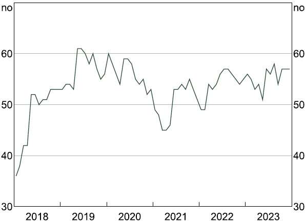
Sources: ABS; Authors' calculations.
A.1.4 CPI weighting
Where appropriate, measures constructed as a part of our analysis are weighted using weights derived from mapping retailer categories to their approximate category matches in the consumer price index. This mapping is shown in Table A2. Where several retailers are part of the same category, we split their category weight evenly amongst them.
| Retailer group | Nearest analogous ABS CPI expenditure groupings | CPI weight used in analysis(a) |
|---|---|---|
| Alcohol | Alcoholic beverages | 5.0 |
| Automotive | Spare parts and accessories for motor vehicles | 0.8 |
| Clothing | Garments | 2.0 |
| Cosmetics | Personal care products | 0.9 |
| Department store | Combination of: household textiles; household appliances, utensils & tools; clothing & footwear | 5.3 |
| Electrical | Combination of: major household appliances; small electric household appliances; audio, visual & computing equipment | 1.9 |
| Eyewear | Accessories | 0.7 |
| Footwear | Footwear | 0.5 |
| Furniture | Furniture | 1.4 |
| Hardware | Combination of: tools & equipment for house and garden; maintenance & repair of the dwelling | 2.5 |
| Homewares | Combination of: household appliances, utensils & tools; household textiles | 2.0 |
| Jewellery | Accessories | 0.7 |
| Magazines | Newspapers, magazines & stationery | 0.4 |
| Pharmaceuticals | Pharmaceutical products | 1.0 |
|
Note: (a) Based on average annual weights for mapped CPI expenditure groupings between 2018 and 2023. Sources: ABS; Authors' calculations. |
||
A.2 Data cleaning
Price changes are measured between two consecutive observations in the dataset and are calculated in log difference terms. For the survival analysis, we drop price observations that may be stale, which we define as when the distance between two price observations is 30 days or more. As noted in Section 4.2, we also drop the first price spell for each item to avoid the possibility of left censoring. Further cleaning of our imputed regular prices series is described in the next section. Apart from these measures, we include all price observations in the dataset.
A.3 Sales algorithm
Firm-reported regular and sales prices are available in our dataset from late 2020. To extend these series back to the start of 2018 and ensure a consistent definition of sales prices across firms, we develop an algorithm that identifies temporary and clearance sales based on observed price patterns.
Our approach follows the methodology introduced by Nakamura and Steinsson (2008) and further developed in Gautier et al (2024). The algorithm classifies price changes as either regular or discount-related by identifying specific patterns in the evolution of advertised prices over time:
- Temporary (or ‘V-shaped’) sales are flagged when the advertised price of an item falls and then returns to an equal or higher level within three months. To ensure any return to full price can be observed for all items, we exclude prices recorded within the last three months in which a firm appears in the dataset.
- A temporary sale flag is removed if a post-discounting price is followed by another price decline within 14 days. This helps to avoid misclassifying volatile pricing behaviour as discounting activity.
- Clearance sales are identified when an advertised price falls by at least 25 per cent and the item exits the dataset within one month. Prices within one month of the end of a firm's data are excluded from the data to ensure the exit condition can be verified.[33]
To assess the performance of the algorithm, we compare our imputed regular and sales prices series to ABS-recorded full and discount prices series available from late 2020 onwards (Figures A3 and A4). The imputed and ABS-recorded series generally align well in level and trend. However, at disaggregated levels, the ABS-recorded data suggest some inconsistencies in how firms distinguish between regular and sales prices, likely reflecting variation in how retailers label discounts on their websites or how the web scraper captured this information.
A key advantage of our algorithm is that it applies a uniform definition of sales events across all firms. By focusing on the underlying structure of price changes – rather than relying on retailer-provided labelling – the algorithm ensures that discounts are identified consistently, regardless of how they are attributed in the source data.
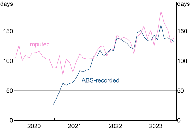
Notes: Item-weighted. Average number of days since prices last changed, conditional on a change having occurred.
Sources: ABS; Authors' calculations.
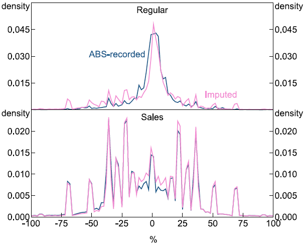
Notes: Item-weighted distribution of log price changes by size estimated by kernel density. The density is evaluated on the x-axes in 2 percentage point intervals. For example, the value plotted around zero corresponds to price changes in the interval –1 to 1 per cent.
Sources: ABS; Authors' calculations.
Footnotes
An example might be two t-shirts in the same style that are different colours. [31]
These are likely to be lower bound estimates for a given item over the sample period, as in an practice items will regularly drop out of the sample as they are retired. [32]
Adjusting the time windows used to identify temporary and clearance sales has only minor effects on our results. [33]