RBA Annual Conference – 2009 Relative Price Shocks, Inflation Expectations, and the Role of Monetary Policy Pierre L Siklos[1]
Abstract
The aim of this paper is to rely on a wide variety of forecasts and survey-based estimates of inflationary expectations since the early 1990s for a group of nine economies, five of which explicitly target inflation, and ask: to what extent are disagreements over forecasts of inflation driven by movements in relative prices? The empirical evidence leads to the following conclusions. First, there is little doubt that inflation targeting has contributed to narrowing the forecast differences vis-à-vis inflation forecasts for the United States. Second, there is some evidence that, at least since 1990, inflation forecasts in the economies considered that had deviated substantially from US forecasts show signs of converging towards US expectations. Third, examining the mean of the distribution of forecasts potentially omits important insights about what drives inflation expectations. Finally, commodity and asset prices clearly move inflation forecasts, although this is a phenomenon of the second half of the sample. Prior to around 1999 relative price effects on expectations are insignificant.
1. Introduction
The last two decades have seen a remarkable convergence in inflation rates around the world. The role that monetary policy plays in achieving this outcome continues to be debated. There is, of course, a long tradition in the profession linking inflation performance to monetary policy. For example, during the depths of the Great Depression, in a landmark 1932 study of commodity prices covering two centuries of data, Warren and Pearson (1932) remarked: ‘Any price level that is out of adjustment with the monetary situation should not be expected to be maintained permanently’ (p 67). A look at any of the recent inflation reports published by several central banks would doubtlessly produce very similar sentiments about the behaviour of inflation. Yet, there is also a case to be made that economists have yet to fully grasp the dynamics of inflation (for example, Bernanke 2008). This state of affairs also carries over to our understanding of what moves inflation forecasts. Adding to the mix, sharp movements in both commodity and asset prices in recent years (see Section 3 below) raise a host of questions about what factors drive expectations of inflation (see also Reis and Watson 2009).
The financial and economic crisis that began in July–August 2007 only deepens the mystery about what influences inflation rates around the world since aggregate price level movements have been relatively benign over the past two years, at least in the industrialised world. There has been no shortage, however, of commentary by central banking officials and other analysts over prospects of a spiralling inflation or deflation.[2] As Trichet (2009) remarked concerning the conduct of monetary policy in turbulent times:
… the evidence supports the view that a central bank's ability to ease monetary conditions – and thereby support the stabilisation of inflation and output – is significantly enhanced by its ability to anchor private expectations.
However, what explains this ability to anchor expectations, and the role played by the monetary policy regime in place, remains open to debate and more research. Therefore, studying the determinants of inflation and, in particular, how relative price shocks interact with inflationary expectations remains an important task.
Adding to the difficulties in our understanding of the inflationary process is the fact that observers of inflation forecasts normally have very little information about the model, or models, that were used to generate a forecast, or the extent to which certain economic variables (for example, commodity prices), as opposed to informed judgment, drive changes in forecasts over time. The problem of identifying the signal from the noise is, of course, an old one.
This paper relies on a wide variety of forecasts and survey-based estimates of inflationary expectations since the early 1990s for a group of nine economies, five of which explicitly target inflation, and asks: to what extent are disagreements over forecasts of inflation driven by movements in relative prices? As there has been considerable interest about whether inflation has been driven by global factors, it is equally important to examine to what extent inflationary expectations are idiosyncratic or driven by factors common to all the economies considered. A variety of subsidiary issues also emerge from the questions that this paper sets out to explore. For example, while small changes in commodity prices may have no significant effect on inflation forecasts, larger changes could have a substantial influence on inflation forecasts. As we shall see, this asymmetric effect appears plausible. In this regard, it is also of interest to examine the extent to which large shocks have permanent or transitory effects on inflationary expectations. Moreover, it is also natural to consider whether these sorts of effects are influenced by the adoption of inflation targeting.
Disagreements about inflationary expectations are almost always defined in terms of a distribution of forecasts prepared in individual countries and are presumably focused on the determinants of the domestic inflationary experience.[3] In the present study I depart from this norm to consider disagreement relative to a different benchmark, namely the US experience. This is done for at least three reasons. First, on both historical and economic grounds, the US experience with inflation remains a useful benchmark, particularly over my sample periods given the earlier success in controlling inflation in the United States. Needless to say, there is considerable debate about the role played by the US Federal Reserve (Fed). While Fed officials have long defended their dual mandate, the recent fashion in central banking and policy-making circles has been to adopt a form of inflation targeting (for example, see Siklos 2009a and references therein). The extent to which this distinction matters is an ongoing research topic. Finally, the decade of the 1990s and early 2000s was a period of substantial globalisation, for both finance and trade. Hence, it is reasonable to posit that inflationary expectations also contain a global element. Consequently, if US inflation and inflation expectations represent a global benchmark, then it is sensible for forecasters, businesses and households to take this information into account perhaps in a more explicit fashion than has heretofore been the case.
An additional contribution of the present study is to generate evidence about the behaviour of inflation expectations by exploiting as broad a sample in terms of the number of forecasts or forecasters as I was able to collect for each economy. Thus, for example, for the United States, Japan, and the euro area, inflation expectations from almost a dozen sources are considered. This comprehensive dataset provides us with some new insights into the behaviour of inflation expectations over time.
The rest of the paper is organised as follows. In the following section I provide a brief overview of the literature linking relative price shocks and central bank strategies to inflation and expectations of inflation. Section 3 introduces the data and provides a bird's eye view of the stylised facts. Section 4 presents some econometric evidence which relies on a variety of techniques, each of which is aimed at providing evidence about the various questions raised in this study. Section 5 concludes. Appendix A documents the inflation forecasts used in this paper and the sources of those forecasts.
2. Relative Price Shocks, Inflation and Monetary Policy
It is perhaps surprising that some prominent economists claim we do not sufficiently understand the dynamics of inflation. Nevertheless, we have learned a great deal about the determinants of inflation over the past decade or so, no doubt assisted by the spread of inflation targeting around the world.[4] What follows then is a concise summary of the existing consensus about some stylised facts.
First, while inflation is persistent, it appears to have fallen substantially in many parts of the world (Benati 2008), possibly more so in inflation-targeting (IT) economies than elsewhere (for example, Siklos 1999a). Whether the combination of lower and more stable inflation has led to expectations of inflation becoming better anchored remains unsettled (for example, Bernanke 2007, Mishkin 2007a, and references therein). Two sets of questions arise here. Can we say whether certain monetary policy regimes (for example, inflation targeting) are better able to hold down inflation expectations than others? If this is the case, what are the sources of disagreements in expectations? It may be that an unstable economic environment leads to persistent deviations in inflation expectations from a path to which the monetary authority plans to adhere. It is also possible that inflation expectations react excessively to relative price shocks, particularly ones that are large and believed to contain a significant permanent component. A relevant consideration here is that the literature has not come to a definitive understanding over how such disagreements are to be measured (for example, see Lahiri and Sheng 2008, and references therein).[5] It should be emphasised at this stage that data limitations pose a serious constraint on the information that can be extracted from inflation forecast and survey data.[6] It is typically the case that point forecasts are used. However, other than for a very few economies (for example, the United States and the United Kingdom), researchers generally do not have access to the distribution of forecasts. This consideration can be crucial since, as shown by Mankiw, Reis and Wolfers (2004), the information content of mean or median forecasts can mask considerable underlying forecast disagreements.[7]
Second, the notion that expectations are rational, which leads to the testable implication that they are both correct, on average, and efficient and unbiased, does imply that there is little additional information that could have been brought to bear to improve on them. It can be said, rather charitably, that this view has received mixed support.[8] In any event, the view that forecasts are rational and/or unbiased contradicts the increased emphasis placed by central banks on improving and intensifying their communication function (for example, Blinder et al 2008). Then there is the literature that points out fairly convincingly not only that learning takes place in any economic environment but that the policy regime itself can assist in the learning process (for example, Sargent 1999 and Orphanides and Williams 2007).
Third, contrary to what one might believe a priori, the low and stable inflationary environment of the past 15 years or so has not necessarily made inflation easier to forecast. Indeed, arguably the most widely used inflation model in the profession, namely a New Keynesian-style Phillips curve, performs rather poorly (for example, Rudd and Whelan 2007 and Stock and Watson 2007) in spite of its strong micro-foundations (for example, Kiley 2008). There continues to be a wide-ranging debate about the links between inflation and inflation expectations, and the relative weight that ought to be placed on certain factors over others. For example, for a time, there was increasingly prominent discussion devoted to the influence of price developments in China as a source for global disinflation (for example, Rogoff 2003, Ball 2006, Borio and Filardo 2007, Ihrig et al 2007 and Côté and de Resende 2008). However, it proves to be extremely difficult to identify a separate role for China from the impact of the global consensus in favour of lower inflation or, for that matter, the role played by institutional mechanisms that ensure that low inflation remains in place (for example, Acemoglu et al 2008, and Bohl, Mayes and Siklos, forthcoming). Beyond these considerations, there is the apparent tenuous connection between expectations and actual inflation rates (for example, Blinder 1999) which must be contrasted with the view that the public does care very much about inflation (for example, Shiller 1997). The relationship between these two crucial variables is further complicated by the evidence that pass-through effects, either via the exchange rate, or through the influence of changes in commodity prices, have diminished considerably in recent years (for example, Hooker 2002 and Gagnon and Ihrig 2004). Interestingly, investigations of the behaviour of commodity prices, for example, and how their movements are linked to ones in aggregate price levels, generally fail to exploit the possibility that the appropriate relationship is asymmetric in nature.[9] Hence, a rise in oil prices might feed into inflation rates more quickly, and remain more persistent, than a reduction in the price of oil.[10]
Brief mention also ought to be made about the horizon over which expectations are evaluated and how these are constructed. Only a handful of industrial countries have developed inflation-indexed bond markets which provide researchers with a source of data on long-run inflationary expectations. Moreover, the extent to which these markets are liquid, and the length of time they have been in place, also pose additional constraints for a cross-country study of the kind undertaken here. It is also the case that there is a paucity of survey or other longer-horizon forecasts for a large cross-section of countries.[11] This is unfortunate since this information directly pertains to the role of the monetary policy regime.[12] Accordingly, the empirical evidence that follows focuses on short-term forecasts. If there is a significant probability that any existing regime will change – a likelihood that may well have risen in some cases in light of the Global Financial Crisis, even though there are few outward signs that policy-makers are contemplating changing their monetary policy regime – then one factor that explains what drives inflation expectations will have been omitted. Otherwise, the empirical evidence below provides some evidence about the role of central banks, their policies, as well as the influence of relative prices, on the evolution of inflationary expectations.
Most studies rely on forecast or expectations data from one or a very small number of sources. For example, an analysis of the properties of inflation forecast errors is usually conducted on a single forecast from a public institution (such as the IMF or the OECD), a private firm (such as Consensus Economics), or a formal survey of forecasters (such as the Survey of Professional Forecasters). It is interesting to consider, however, whether the source provides any additional clues about what drives the forecasts and this study is an attempt to do so.[13]
Finally, there has been considerable debate about the desirability of the central bank publishing its own forecasts. There is no consensus about this question and it is inappropriate here to delve into the relevant issues (see, however, Mishkin 2007b, Ch 5). Nevertheless, it is worth considering such forecasts as well. They, together with forecasts from other sources, provide indirect clues about whether, ex post, prior beliefs about differences in information sets that go into producing such forecasts explain how well expectations are anchored. They also provide clues about how sensitive forecasts may be to the different pressures on inflation over time, including those stemming from relative price changes, the monetary regime in place, as well as some of the other factors noted above.
3. A Bird's Eye View of the Data
Appendix A provides details of the data sources and definitions used in this study. All tests and estimates are based on data converted to a quarterly frequency. Original forecasts are monthly (M), quarterly (Q) or half-yearly (H). Generally, the sample covers the period 1990 to 2008. Inflation is defined in terms of the headline rate for the CPI for all the economies considered, expressed in annualised terms. The empirical evidence shown below examines the experience of five IT economies – Australia, Canada, New Zealand, Sweden and the United Kingdom – and four non-IT economies – the euro area, Japan, Switzerland and the United States. The expectations data are time series of current-year and one-year-ahead forecasts. Three types of forecast data are used: professional forecasts; forecasts derived from survey data; and any available central bank forecasts.
There are several difficult issues that arise when resorting to these data. First, most of the forecasts are for the calendar year. For example, each month (usually around the third week of the month) The Economist publishes private-sector forecasts of inflation (and real GDP growth) for the current and following calendar years (one-year-ahead forecasts). Other forecasts are presented in a similar manner (for example, Consensus forecasts). Some forecasts (those of the OECD, for instance) are published semi-annually while others (for example, the RBNZ) release forecasts on a quarterly basis.[14] As a result, there is both an issue of timing and the horizon to which the forecast pertains. Studies that rely on these data are aware of this, but adjustments to correct for such problems are often ad hoc or are said to have little influence on the outcome of empirical tests. Given the persistence properties of inflation, it is conceivable that calendar-year forecasts pose little difficulty. In what follows, no special adjustments are made to the data. While some experiments were conducted to determine how large the resulting biases might be, it appears (in line with other studies) that they do not appear to be large.[15]
In the case of survey data, the researcher faces the additional difficulty that the data are not always presented in the form of an inflation rate. Instead, many surveys (for example, those of the European Commission and the Centre for European Economic Research (ZEW)) report an index. Generally, the literature has adopted two approaches to convert the data into usable form. Smith and McAleer (1995) provide a nice survey of the methodologies originally due to Carlson and Parkin (1975) and Pesaran (1985, 1987). The former is generally referred to as the probability approach, whereas the latter is a regression-based technique used to convert an index into an estimate of inflation expectations. Both techniques were implemented in this study and readers are referred to the relevant papers for additional details.
A final comment concerning forecasts is also in order. While the measurement of forecast disagreement used in this study treats all forecasts on an equal footing, the researcher does not observe the objective function implicit in the construction of these forecasts, that is, whether the aim of the forecaster is to find the best forecast of inflation or one that might attract the greatest public attention. The implications are not formally explored in this study but should be borne in mind in future extensions of the present research.
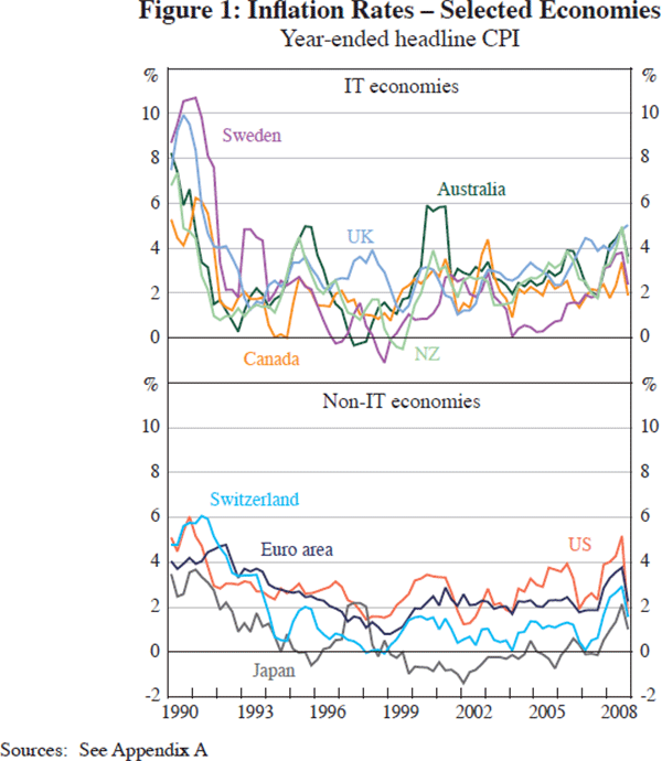
Consider first overall inflation performance, as shown in Figure 1. The top and bottom panels show CPI inflation in the IT and non-IT economies, respectively. There is little evidence of notable differences between IT and non-IT economies' inflation rates in the period since inflation targeting was adopted. Prior to 1994, however, one does clearly see the rapid disinflation that took place in the IT camp.[16] As will be seen below, appearances can be deceiving as some persistent differences in overall inflation performance between the IT and non-IT economies can be observed. The figure also highlights why there is continuing debate not only about the relative superiority of an IT regime but also whether forces more global in nature, including commodity price movements, are driving inflation rates around the world.
Figures 2 and 3 plot a number of commodity and asset prices.[17] These do not exhaust the set of relevant commodity prices that may have affected inflation expectations over time in each of the economies considered. Nevertheless, the various series shown are fairly representative of the data that various authors in the relevant literature have used to investigate the macroeconomic role of commodity and asset prices.[18] The series displayed in the figures consist of individual commodity price indices as well as aggregate commodity price indices that some of the central banks in our sample publish and monitor on a regular basis. The variability of commodity prices (Figure 2) is quite apparent. Nevertheless, it is usually the case that broader indices of commodity prices are relatively less volatile than many of the individual commodity prices sampled. In addition, most of the series appear to be mean-reverting and there is also a visual hint at least of some asymmetry in commodity price movements (somewhat steadier increases and more rapid decreases). Formal testing of the statistical properties of these series follows below.
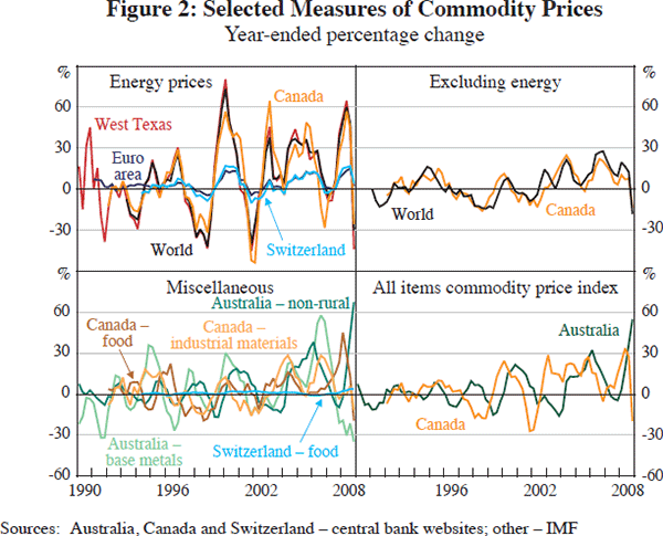
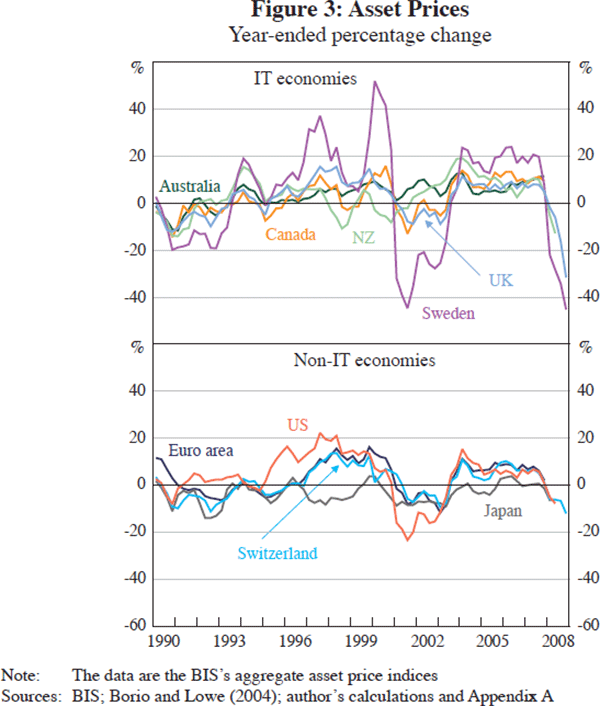
Figure 3 plots the rate of change in the BIS's aggregate asset price index (Borio and Lowe 2004) for the IT and non-IT group of economies in our example. One can interpret fluctuations in these indices as a relative price of sorts – that is, for current versus future consumption. Alternatively, movements in these indices may provide clues about imbalances in the economy to which monetary policy and, presumably, inflation expectations, might react. The plots suggest considerable variability in asset prices in all the economies considered, although, on balance, volatility appears relatively larger in the IT economies. Also notable is asymmetry in growth rates of asset prices, with the exception of the Japanese experience.[19]
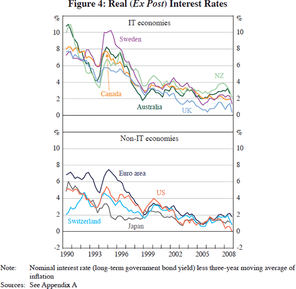
Figure 4 plots an estimate of the real interest rate based on the difference between the nominal long-term government bond yield and a three-year moving average of inflation. Needless to say, there is considerable debate about the proper measurement of real interest rates, let alone how to proxy longer-term expectations of inflation. Nevertheless, while estimates of the real interest rate may vary depending on the details of the calculations, it is likely that the series shown in Figure 4 offer a fair portrayal of how the stance of monetary policy has evolved across the economies considered since 1990.[20] During the first half of the 1990s, real interest rates were relatively higher in the IT group of countries. As several authors have suggested, this stylised fact captures both the adjustment towards a lower inflation rate the newly IT countries were aiming for at the time, as well as an expression of the attempt by these central banks, given their historical experience with inflation, to establish bona fides in delivering inflation control. However, by the late 1990s it generally becomes difficult to distinguish the stance of monetary policy in IT economies from that in non-IT economies. This feature of the data also captures the stalemate in the debate between supporters of inflation targeting and others who have found it difficult to see, or are sceptical of, the superiority of one type of policy regime over another.
I now turn to some stylised facts about inflation expectations. Figure 5 plots CPI inflation in the IT economies on the horizontal axis against various available measures of one-year-ahead inflation expectations (see Appendix A for details).[21] The same plots are generated for the non-IT economies in Figure 6. As noted previously, it is useful to distinguish between a general disinflationary phase versus a period when inflation remained relatively low and stable. Clearly, it is not straightforward to identify any such ‘break’ over the period examined. Moreover, it is likely to be difficult to pinpoint a common break across the nine economies considered in this study. Hence, I compare the full sample (1990–2008) to a sub-sample consisting of observations for the 1999–2008 period.[22] Most observers would agree that by that time all IT regimes were in place long enough to avoid problems arising from initial conditions biasing the results in favour of inflation targeting. Accordingly, the left-hand-side panels display the evidence for the full sample while sub-sample results are summarised in the right-hand-side panels. There are three notable features about the simple relationship between inflation and inflation expectations displayed here. First, with the possible exception of New Zealand, the country that first adopted inflation targeting in 1990, higher current inflation is generally associated with a rise in one-year-ahead inflation. The same relationship is apparent for Switzerland and Japan, but somewhat less so for the other non-IT economies. Second, the relationship between inflation and one-year-ahead expectations is considerably tighter after 1999 in the IT group of countries. This phenomenon is less apparent among the non-IT economies, except for Switzerland, who is not an inflation targeter but does target a forecast for inflation. The apparent clustering of inflation and inflation forecasts is suggestive of an anchoring of inflation expectations and the change is most visible among the IT group of countries. Whether inflation targeting alone, or in combination with other factors, can explain the difference is, of course, an empirical question. Finally, regardless of the nature of the monetary policy regime, there are fewer ‘outliers’ after 1999 in the various scatter plots shown. This suggests that the era since 1999 is, broadly speaking, characterised by fewer inflation surprises.
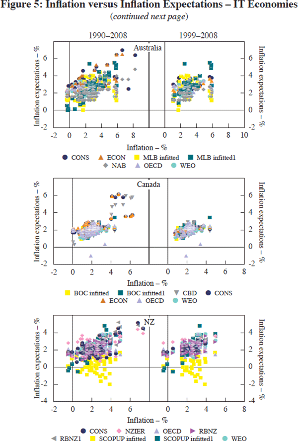
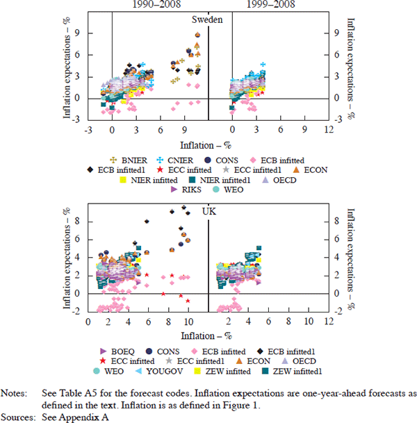
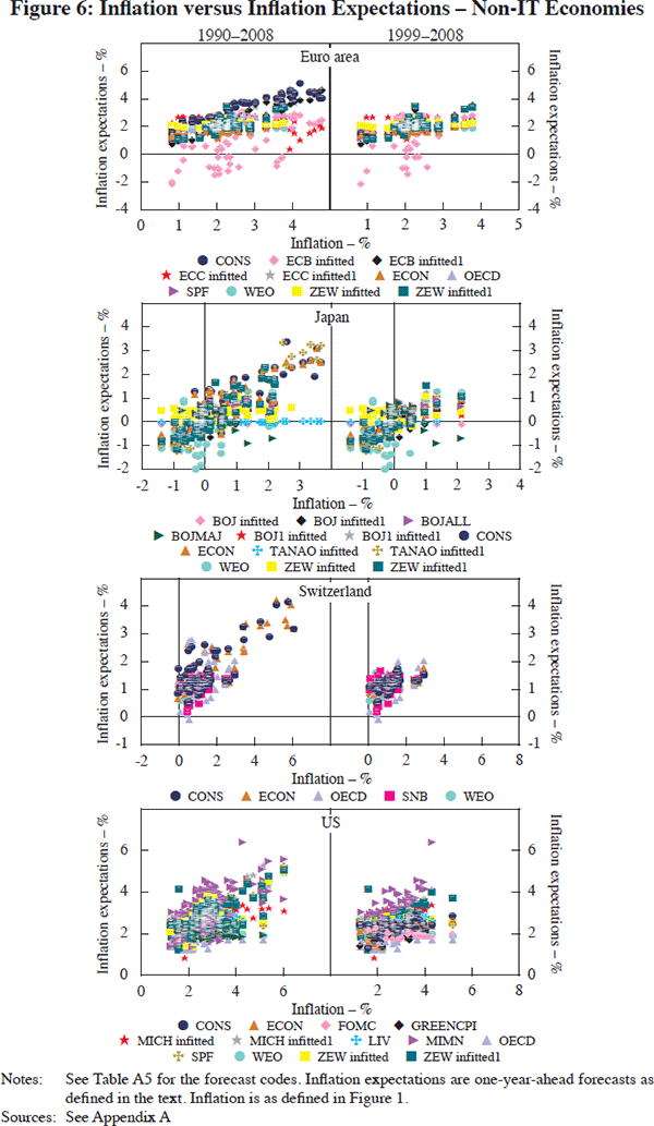
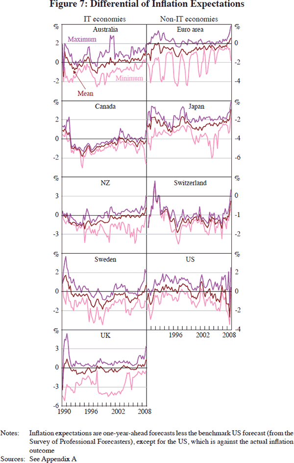
Figure 7 displays evidence of the range of inflation expectations across economies and sources of data. As noted previously, it is customary to examine inflation forecasts or surveys relative to some domestic benchmark. However, since this study partly aims to assess the role of global forces on inflation, as proxied by the US experience, the figure shows differences in expectations relative to a US benchmark.[23] Examination of the data in Figure 7 suggests that in at least three of the five IT economies (Australia, Canada and Sweden), the differences vis-à-vis one-year-ahead US inflation forecasts have diminished somewhat over time while a similar pattern is less apparent for New Zealand and the United Kingdom. Equally interesting is the fact that inflation expectations are persistently below those of the United States, especially beginning in the mid 1990s, except possibly for the United Kingdom. It seems then that there is both a global element to the determination of inflation expectations (what one might loosely call a trend component) and a domestic component suggestive of the decoupling of these expectations relative to the United States, perhaps due to the adoption of inflation targeting. As seen in Figure 7, no such interpretation is evident for the non-IT economies in the sample. The idiosyncratic experience of Japan is evident, while there is seemingly little change in the behaviour of expectations in Switzerland relative to the United States. Only the euro area begins to resemble the US experience and this may point toward the success of the fledgling central bank in anchoring expectations to levels comparable to ones exhibited in the United States.
Finally, Figure 8 plots our measure of forecast disagreement for each of the nine economies in this study. The shaded areas highlight, where relevant, the period before inflation targets were introduced.[24] As noted previously, there is no universally agreed-upon measure of forecast disagreement. However, some researchers typically resort to the following definition

where: d is the measure of disagreement for a particular country;
Fith is the i-th forecast for horizon h
at time t; and  is the mean across the N
available forecasts for that
country.[25]
To highlight the evolution of disagreement over time, Equation (1) is evaluated in
a five-year rolling
sample.[26]
In what follows, h is always set to 1 to indicate that the focus is
on one-year-ahead forecasts. The results indicate that in all IT economies,
disagreement tended to rise in the early phases of the new monetary policy
regime. Nevertheless, the rise is typically very brief in duration with the
possible exception of New Zealand where disagreement increased over a six-year
period. In contrast, disagreement rose over five years in Australia, two years
in the United Kingdom, and one year in Canada. Arguably, the ‘shock’
associated with the change in monetary policy regime was greatest for New Zealand.
It is notable as well that disagreement tends to fall sharply in some cases
following the adoption and adjustment to the IT regime.
is the mean across the N
available forecasts for that
country.[25]
To highlight the evolution of disagreement over time, Equation (1) is evaluated in
a five-year rolling
sample.[26]
In what follows, h is always set to 1 to indicate that the focus is
on one-year-ahead forecasts. The results indicate that in all IT economies,
disagreement tended to rise in the early phases of the new monetary policy
regime. Nevertheless, the rise is typically very brief in duration with the
possible exception of New Zealand where disagreement increased over a six-year
period. In contrast, disagreement rose over five years in Australia, two years
in the United Kingdom, and one year in Canada. Arguably, the ‘shock’
associated with the change in monetary policy regime was greatest for New Zealand.
It is notable as well that disagreement tends to fall sharply in some cases
following the adoption and adjustment to the IT regime.
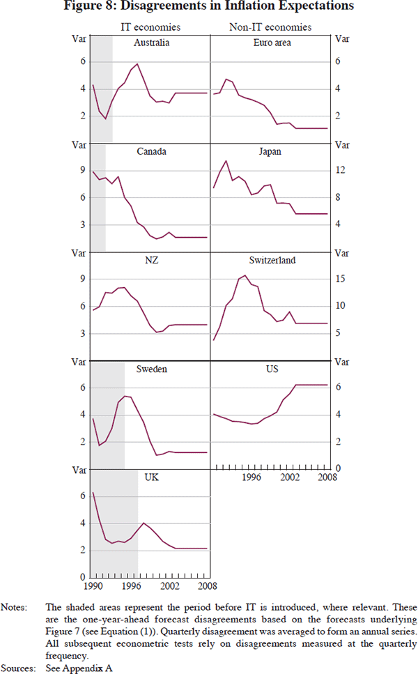
Comparisons with the record of forecast disagreement in non-IT economies are particularly instructive. Disagreement in the euro area rises over a three-year period then permanently falls, but what is most notable is that disagreement falls around the start of European Monetary Union (EMU). Contrast this with the Japanese experience, which shows a period of elevated disagreement essentially covering the so-called ‘lost decade’ before falling since the turn of the century. The experience of Switzerland reveals a sharp rise in forecast disagreement during the first half of the 1990s and, in spite of a small dip in the second half of that decade, disagreement remains permanently higher than at the beginning of the sample. There is a less dramatic but equally pronounced rise in forecast disagreement in the United States, with estimates of disagreement for the most part increasing steadily until 2002. Clearly, there is considerable diversity in the forecasting experience across this sample of economies, but one should not exaggerate the differences. After all, every single economy in the sample experiences a rise in forecast disagreement sometime during the 1990s precisely when central banks in the industrial world, whether they formally targeted inflation or not, emphasised the desirability of low and stable inflation. It is likely that changes in monetary policy credibility, the actual design and implementation of inflation control strategies, as well as the international environment, have each played a role in the emergence and subsequent reversal of these forecast disagreements. I now turn to some preliminary evidence estimating the significance of some of these factors.
4. Empirical Evidence
Table 1 provides some summary statistics about the stationarity, or otherwise, of the key series under investigation. The top portion of the tables presents panel unit root tests. The two most widely used tests, namely those of Levin-Lin-Chu (LLC) and Im-Pesaran-Shin (IPS), are reported.[27]
| A. Panel unit root test: cointegration of domestic and US forecasts | |||
|---|---|---|---|
| LLC | IPS | Observations | |
| Australia I | −2.44 (0.01) | −3.47 (0.00) | 425 |
| Australia II | −2.55 (0.01) | −3.77 (0.00) | 192 |
| Combined | −2.83 (0.00) | −3.72 (0.00) | |
| Canada I | −4.09 (0.00) | −5.84 (0.00) | 375 |
| Canada II | −3.33 (0.00) | −4.72 (0.00) | 188 |
| Combined | −4.10 (0.00) | −5.84 (0.00) | |
| New Zealand I | 0.52 (0.70) | −0.70 (0.24) | 454 |
| New Zealand II | −3.81 (0.00) | −4.70 (0.00) | 157 |
| Combined | 0.53 (0.70) | −0.70 (0.24) | |
| Sweden I | −1.36 (0.09) | −3.49 (0.00) | 621 |
| Sweden II | −3.10 (0.00) | −3.62 (0.00) | 174 |
| Combined | −1.36 (0.09) | −3.49 (0.00) | |
| United Kingdom I | −2.97 (0.00) | −4.94 (0.00) | 746 |
| United Kingdom II | −4.35 (0.00) | −4.53 (0.00) | 299 |
| Combined | −2.97 (0.00) | −4.94 (0.00) | |
| Euro area I | 0.28 (0.61) | −1.32 (0.09) | 629 |
| Euro area II | −3.87 (0.00) | −4.03 (0.00) | 200 |
| Combined | 0.28 (0.61) | −1.32 (0.10) | |
| Japan I | 0.49 (0.69) | −1.47 (0.07) | 593 |
| Japan II | −4.51 (0.00) | −4.25 (0.00) | 283 |
| Combined | 0.49 (0.69) | −1.47 (0.07) | |
| Switzerland I | −0.04 (0.49) | −2.82 (0.00) | 257 |
| Switzerland II | −3.94 (0.00) | −5.35 (0.00) | 213 |
| Combined | −0.04 (0.49) | −2.82 (0.00) | |
| United States I | 1.24 (0.89) | −7.62 (0.00) | 756 |
| United States II | −2.70 (0.00) | −7.05 (0.00) | 504 |
| Combined | 1.24 (0.89) | −7.62 (0.90) | |
| B. Threshold cointegration tests | |||||
|---|---|---|---|---|---|
| ρ1 | ρ2 | F1 | F2 | τ | |
| Australia | −0.02 (0.05) | −1.74 (0.17) | 49.55* | 89.25* | −0.30 |
| Canada | −0.09* (0.04) | −0.28 (0.13) | 4.45* | 2.02 | −0.62 |
| New Zealand | −0.02 (0.06) | −0.53* (0.24) | 9.47* | 6.02 | −0.84 |
| Sweden | −0.11* (0.04) | 0.28 (0.14) | 5.24* | 7.03* | −0.65 |
| United Kingdom | −0.04 (0.05) | −1.14* (0.10) | 60.75* | 89.52* | −0.64 |
| Euro area | −0.05 (0.08) | −0.82 (0.17) | 12.43* | 17.89* | −0.64 |
| Japan | −0.19* (0.08) | 1.06 (1.42) | 2.91* | 0.77 | −2.35 |
| Switzerland | −0.16* (0.07) | −1.10 (0.45) | 5.84* | 4.35 | −1.05 |
| United States | −0.09 (0.06) | −1.63* (0.15) | 24.06* | 38.94* | −0.85 |
| C. Unit root tests: commodity and asset prices | |||
|---|---|---|---|
| ERS (ADF) | LLC | IPS | |
| Energy | 3.13 (0.99) | 1.06 (0.86) | |
| Brent | −1.56 (5) | ||
| West Texas | −1.50 (5) | ||
| Canada | −1.68 (4) | ||
| New Zealand | −1.06 (3) | ||
| Switzerland | −1.43 (6) | ||
| World | −1.47 (5) | ||
| Other commodities | 4.37 (1.00) | 2.79 (0.99) | |
| Metals | −2.45 (2) | ||
| Non-rural | −0.79 (1) | ||
| Canada – food | −2.70 (1) | ||
| Switzerland – food | −2.17 (3) | ||
| Australia – total | −0.69 (1) | ||
| Canada – total | −1.77 (2) | ||
| Canada – non-energy | −2.32 (4) | ||
| World – non-fuel | −2.50 (7) | ||
| Asset prices | 0.001 (0.50) | −0.09 (0.47) | |
| Aggregate | 2.61 (0.99) | 3.50 (0.99) | |
| Australia | −0.14 (2) | ||
| Canada | −1.74 (1) | ||
| New Zealand | −2.69 (8) | ||
| Sweden | −2.34 (2) | ||
| United Kingdom | −2.42 (1) | ||
| Euro area | −2.02 (12) | −1.12 (0.13) | −1.41 (0.08) |
| Japan | −1.25 (4) | −1.49 (0.13) | 0.29 (0.62) |
| Switzerland | −3.17 (4) | ||
| United States | −2.32 (4) | ||
| Equities | −1.43 (0.08) | −2.84 (0.00) | |
| Australia | −1.50 (1) | −0.87 (0.19) | −1.16 (0.12) |
| Canada | −2.23 (1) | ||
| New Zealand | −2.51 (11) | ||
| Sweden | −1.83 (5) | ||
| United Kingdom | −1.72 (1) | ||
| Euro area | −1.75 (3) | −0.18 (0.43) | 0.36 (0.64) |
| Japan | −2.01 (3) | −1.52 (0.07) | −1.14 (0.13) |
| Switzerland | −1.26 (1) | ||
| United States | −1.40 (1) | ||
| Housing | −3.26 (0.00) | −0.49 (0.31) | |
| Australia | −1.35 (1) | ||
| Canada | −1.83 (8) | ||
| New Zealand | −2.35 (1) | ||
| Sweden | −1.49 (3) | ||
| United Kingdom | −1.31 (1) | ||
| Euro area | −2.30 (4) | ||
| Japan | −1.77 (4) | ||
| Switzerland | −0.72 (2) | ||
| United States | −4.04 (4) | ||
| Notes: In Part A, the test statistic is shown with p-values in parentheses; italicised numbers are those with p-values that are larger than 0.05 to identify cases where the null is rejected. I refers to non-survey-based forecasts while II refers to the group of survey-based forecasts. Part B gives the estimates of the error correction terms, the test for asymmetry (F1) and the test for whether both error correction terms are jointly equal to zero (F2). The test specification is from Enders and Siklos (2001). * indicates rejection at the 5 per cent significance level. In Part C, the column labelled ERS (ADF) gives the lag length used in the lag augmentation portion of the test equation, chosen according to the Schwarz information criterion (ERS = Elliot-Rothenberg-Stock test). Otherwise, p-values are shown in parentheses in the remaining columns along with the test statistic. A trend was not included in the test specifications. | |||
Both panel tests are essentially versions of the well-known Augmented Dickey-Fuller (ADF) test that would be applied to time-series data for individual countries. The test equation in a panel setting (omitting constants and deterministic components) is written

where: j identifies the particular economy in the sample; and y is the differential between domestic forecasts and the US benchmark forecast. The unit root test statistic then consists of the sample mean of the ADF t-statistics. IPS (2003) provide the critical values. The ADF tests tend to have a downward bias, which is corrected for when a panel test is used. Generally, if all independent parameter estimates are unbiased, then the mean of these estimates is also unbiased (Enders 2004, p 225). Notice that the test based on Equation (2) estimates a unit root test statistic for each cross-section, as well as a country-specific lag augmentation term. In contrast, if the hypothesis that αj ≠ αj', where j ≠ j', cannot be rejected, then an alternative specification of Equation (2), where α and β are fixed across all countries, results in the so-called LLC (2002) panel unit root test.[28] Since the panels considered refer to the differential between domestic forecasts and a US forecast, the test also amounts to asking whether cointegration holds between the various individual forecasts and the representative US forecast. Panels are also subdivided according to whether the forecast is survey-based or not.
In the case of the threshold cointegration test, attention focuses on the stationarity of the individual series of mean domestic forecasts versus the benchmark US forecast. While the benefits of panel estimation are lost, it is possible to determine whether cointegration is a feature of the data once we permit the error correction term to adjust in an asymmetric fashion.[29] The remainder of the table presents various unit root and panel unit root tests for commodity and asset prices. Asymmetric unit root tests are omitted, as the discussion in the previous section made clear the presence of asymmetric behaviour in these time series.
The null of no cointegration is rejected in most cases. In the case of IT regimes, the only exception is for New Zealand forecasts that are not survey-based. The results are mixed for non-survey-based forecasts for Sweden with the LLC test leading to a non-rejection, unless of course one wishes to adopt a 5 per cent critical value, in which case Sweden's non-survey-based forecasts are cointegrated with US forecasts. Turning to the non-IT economies, there are many more rejections of the no cointegration null. This is the case, regardless of the testing procedure employed, for non-survey-based forecasts for the euro area and Japan. The results are more mixed for non-survey-based forecasts for Switzerland and the United States. Therefore, there is some evidence that forecast dispersion behaviour is not the same in IT versus non-IT regimes. It is also interesting to note that the null of no cointegration is never rejected for survey-based forecasts. When the panel stacks together both survey- and non-survey-based one-year-ahead forecasts, the null of no cointegration is almost always rejected. The only exception is New Zealand, although once again the results for the non-IT economies are sensitive to the assumption of a common unit root in the test specification.
If we permit asymmetric adjustment of the momentum-threshold variety, the bivariate cointegration tests suggest that the cointegration property tends to hold. This result holds in five of the nine economies considered, but for this type of cointegration there is no obvious evidence of a distinction between IT and non-IT economies. Further, in absolute value, the attractor toward cointegration is always stronger from below the threshold than from above. This implies that a negative change in the error correction term, explained either by a rise in US inflationary expectations or a fall in the forecast for domestic inflation, exerts a relatively stronger pull than changes in the other direction. Of course, not all cases are statistically significant and, indeed, there are four cases (Canada, Sweden, Japan and Switzerland) where the attractor in the other direction exerts a stronger pull back to equilibrium. It is important to underscore that these results are based on mean forecasts. Consequently, some information is lost and, as shall be seen below, the interpretation of what moves inflationary expectations may be affected by this choice.
Turning to commodity and asset prices, it is not surprising that individually these series exhibit the unit root property. This much should have been apparent from the earlier discussion. Stacking all commodity prices in a panel does not change the conclusions. The same conclusion is reached for the BIS's aggregate asset price indices, although the results are somewhat sensitive in the case of non-IT economies, assuming a 10 per cent critical value is adopted.
Since a fairly large number of individual forecasts were retained for each economy,[30] a natural question to ask is how important is the relative information content of the individual forecasts. While there are many ways of addressing the issue, Table 2 provides summary information of a principal components analysis of the various available forecasts on an economy-by-economy basis.[31] The second and third columns of Table 2 shows the most important forecasts based on the estimated eigenvalues, measured on the basis of explanatory power (as a proportion of the total value). The second column lists the forecasts that would have the greatest weight if a linear combination of forecasts were used instead of, say, a simple mean of available forecasts. There are at least two notable features in the results. First, in practically all cases, either Consensus, The Economist forecasts, or both, are among the first or second principal components of the forecasts. Second, most forecasts contribute a relatively small fraction of the total variation. Consequently, there is no such thing as a dominant forecast. Indeed, it is often the case that at least four to five forecasts are needed to explain close to two-thirds of the variation in one-year-ahead inflation forecasts.
| Economy | Principal component (PC) | Proportion of total variation (%)(a) |
|---|---|---|
| Australia | ECON, OECD, CONS, NAB | 0.37, 0.18, 0.16, 0.09 |
| Canada | PC1: ECON, CONS, BOC, WEO PC2: CBD, BOC, OECD |
0.39, 0.20, 0.14, 0.12, 0.07 |
| Euro area | ECB(2), SPF, OECD, ECC(2), CONS, ECON | 0.41, 0.20, 0.09, 0.09, 0.06, 0.05 |
| Japan | TANAO(2), ZEW(2), CONS, ECON | 0.36, 0.21, 0.12, 0.09 |
| New Zealand | RBNZ, CONS, RBNZ-Survey | 0.47, 0.16, 0.14 |
| Sweden | NIER(2), CONS, ECON, RIKS | 0.52, 0.15, 0.10, 0.07 |
| Switzerland | CONS, ECON, SNB, OECD | 0.55, 0.17, 0.14, 0.10 |
| United Kingdom | PC1: ECC(2), ECB(2), ZEW(2), YOUGOV PC2: ECON, BOE, CONS |
0.29, 0.20, 0.13, 0.08 |
| United States | ECON, CONS, SPF, LIV | 0.40, 0.15, 0.13, 0.07, 0.07 |
| Notes: PC: (1) = probability approach; (2) = regression approach. See
Table A5 for the forecast codes. (a) Eigenvalues |
||
Finally, we turn to some regression estimates of the determinants of the forecast differential. Once again, to conserve space, only a selection of the results are displayed in Table 3.
The estimated specification is a straightforward one and, as such, imposes restrictions that future research will need to consider. I am interested in the determinants of the differences between forecasts of one-year-ahead inflation in economy i, at time t, generated by forecaster j, and the US forecast (SPF). The resulting relationship can be expressed as

where: fd represents the difference between forecaster j's one-year-ahead forecast for economy i at time t and the benchmark US forecast (SPF); A and B are fixed effects; X is a vector of control variables; and, since we are interested in, among other questions, the impact of inflation targeting, I is a dummy variable for this policy regime. One immediate difficulty, noted earlier, is that we are unlikely to have ample information on controls for each country. Moreover, as discussed in Bertrand, Duflo and Mullainathan (2004), standard errors from OLS estimation of Equation (3) can be distorted. Among the possible solutions is to estimate Equation (3) at the economy-wide level, in which case many more covariates are available. This is the strategy adopted below. In addition, as pointed out previously, there is potentially a loss of information when focusing only on the mean value of fd. Hence, three set of results are shown in Table 3. Estimates of Equation (3) for the mean, the lowest (MIN) and highest (MAX) forecast differential are presented. One may view the MIN estimates as proxying the reactions of those who are most optimistic about future domestic inflation while the MAX estimates capture the most pessimistic forecasts.[32] In addition, two sets of sub-sample estimates are provided as it is likely, based on the stylised facts, that the behaviour of inflation and inflation expectations may well have undergone a change around 1999 to 2001.[33] Sub-sample estimation also permits the addition of another variable that is labelled ‘news’. Various dummy variables are constructed (see Appendix A for details) that are set to 1, and are otherwise set to 0, when headlines, primarily in the financial press, highlight a rising fear of future inflation, future rises in the policy interest rate, a future recession or a depreciation of the US dollar – that is, there are separate dummy variables for each of these types of news events.
The vector X consists of the following variables. Oil and commodity prices are proxied by the world price of Brent crude and a world index of non-fuel prices. Both series are in HP-filtered form.[34] Asset prices, namely housing and equity prices that exceed or fall below some HP-filtered trend, are also included. Next, for reasons discussed above, I allow for asymmetric type of adjustment by creating a variable that is set to 1 when the change in the mean differential is greater than zero and is zero otherwise. This gives the opportunity to ascertain whether large positive or negative movements in domestic inflation forecasts relative to the US benchmark measure have a separate impact on fd. The specification also allows for uncertainty, proxied here by the kurtosis (KURT) in the distribution of forecast differential, as well as disagreement in the forecasts (DIS), to influence fd.[35] These variables not only capture the role of second and third moments but, in so doing, include some distributional information, omitted in the process of aggregation. Finally, other than a lagged dependent variable, included to measure persistence in fd, a variable that measures how long a country has been in an IT environment is also included (ITDUR).
It is clear from the estimated coefficients that our suspicion that something changed around 1999 to 2001 is borne out.[36] For example, the asymmetry found for the 1990–2008 sample, where a rise in the inflation forecast differential is reversed (but not vice versa), is not apparent in the most recent period. Second, uncertainty about future inflationary expectations are statistically significant in the sub-samples but not in the full sample. Finally, and perhaps most interestingly, relative prices, as proxied by oil, housing and equity prices, are not statistically significant in the full sample but have a clear impact in the sub-sample estimates shown.
The results for the lowest (MIN) and highest (MAX) imply some rather interesting and important differences vis-à-vis the panel estimate based on the mean. First, notice that the IT dummy is statistically significant in both cases. In addition, at both ends of the distribution, as it were, we find that the introduction of inflation targeting reduces the differences in one-year-ahead inflation forecasts by 0.17 per cent. This is only trivially offset by the length of time the country in question has been targeting inflation (ITDUR). Next, it is clearly the case that the high level of persistence found for the mean-based estimates is more a feature of the ‘pessimists’ among the group of forecasters than for the ‘optimists’, with the latter specification yielding significantly lower persistence in the forecast differential (0.59 versus 0.75). In contrast, optimistic forecasters are relatively more worried about future uncertainty, which tends to narrow inflation forecast differentials. Similarly, disagreement among forecasters has twice as large an effect on the forecast differential when the forecast is a relatively optimistic one.
Before concluding, it is worth delving into the changing persistence properties of the forecast differential and the role of inflation targeting in the individual economies in the sample. To do this, a version of Equation (3) is estimated for each economy separately (not shown) and Table 4 summarises what happens to the estimates of persistence as well as the IT dummy. It is rather striking that the full sample sees all coefficients highly significant while every single coefficient in both sub-samples shown are statistically insignificant at the 5 per cent level. This result is to be expected since, as noted previously, much of the disinflation was achieved by the mid 1990s.[37] Just as with headline inflation, there is effectively much less persistence in inflation forecasts in the more recent sample period. While it is plausible to suppose that forecasters are now less backward-looking, the robustness of this result has yet to be properly tested. To be sure, there are differences in the estimates and clearly one can imagine specifications similar to Equation (3) that are equally plausible. However, some of the results in Table 4 do not seem to be greatly at variance with the summary estimates provided in Table 3. Of the five IT economies, separate estimates of δ (the coefficient on the IT dummy variable) can be provided for in only four cases. The results suggest that the reduction in the forecast differential due to inflation targeting is primarily a feature of the Canadian and Swedish experiences but not of Australia and the United Kingdom.
| Economy | Full: 1990–2008 | 1999–2008 | 2001–2008 | Inflation targeting |
|---|---|---|---|---|
| Dependent variable: Mean fdt | ||||
| Australia | 0.46* | 0.05 | −0.12 | 0.03 (0.86) |
| Canada | 0.70* | −0.09 | 0.22 | −0.28 (0.07) |
| New Zealand | 0.54* | −0.35 | 0.02 | na(b) |
| Sweden | 0.84* | 0.29 | 0.63 | −0.18 (0.10) |
| United Kingdom | 0.46* | 0.17 | 0.15 | 0.15 (0.29) |
| Euro area | 0.55* | −0.26 | −0.27 | na |
| Japan | 0.78* | 0.47(a) | 0.44 | na |
| Switzerland | 0.88* | 0.18 | 0.25 | na |
| United States | 0.39* | 0.29 | 0.36 | na |
| Notes: The first three columns give the coefficient estimates and * indicates
statistically significant at the 5 per cent level. The last column gives
the estimate of the response to the IT dummy (see Equation (3) for the
panel version of the same specification). p-values in parentheses.
(a) p-value is 0.10. (b) New Zealand introduced inflation targeting in 1990:Q1. |
||||
5. Conclusions
This paper began by noting that there is still much to be learned from analysing the behaviour of inflation expectations. In contrast with most studies of this kind, the strategy followed here is to extract information contained in the reasonably large variety of inflation forecasts. I then considered how forecasts in five IT and four non-IT economies have evolved since the early 1990s. What can we make of the results? First, there is little doubt that inflation targeting has contributed to narrowing the forecast differences vis-à-vis US inflation forecasts. Second, there is some evidence that, at least since 1990, inflation forecasts in the economies considered that deviate considerably from US forecasts show signs of converging towards US expectations. Third, examining the mean of the distribution of forecasts potentially omits important insights about what drives inflation expectations. Finally, commodity and asset prices clearly move inflation forecasts, although this is a phenomenon of the second half of the sample. Prior to around 1999, relative price effects on expectations are insignificant.
There is clearly scope for more research. It is unclear whether the specification used is the best one for extracting all of the useful information contained in the dataset. In addition, one may wish to examine the behaviour of forecasts using a different metric than the one employed here. Finally, one may consider some interaction effects and add some other omitted variables in Equation (3). For example, inflation targeting may operate jointly to reduce inflation forecast uncertainty and disagreement among inflation forecasts. In addition, central banking in the 1990s has been marked by a trend towards greater transparency. Explicit accounting for this characteristic would be useful. These are only a few of the many avenues open for future research.
Appendix A
| Economy | Forecast | Horizons(a) | Start | Survey | Horizons(a) | Start |
|---|---|---|---|---|---|---|
| Australia | ECON | cy, 1y | 1990:M8 | MLB | ya–balance(b) | 1993:Q2 |
| CONS | cy, 1y | 1990:M1 | ||||
| WEO | cy, 1y | 1993:H1 | ||||
| OECD | ya | 1990:H1 | ||||
| Canada | ECON | cy, 1y | 1990:M8 | BOC | 2y–bins(b) | 2001:Q2 |
| CONS | cy, 1y | 1989:M10 | ||||
| WEO | cy, 1y | 1993:H1 | ||||
| CBD | cy, 1y | 1990:Q1 | ||||
| OECD | ya | 1990:H1 | ||||
| Euro area | ECON | cy, 1y | 1998:M11 | SPF | cy, 1y, 2y, 5y | 1999:Q1 |
| CONS | cy, 1y | 1989:M10 | ECB/ECC | ya–balance(b) | 1985:M1 | |
| OECD | ya | 1990:H1 | ZEW | ya–bins(b) | 1991:M12 | |
| Japan | ECON | cy, 1y | 1990:M8 | ZEW | ya–bins(b) | 1991:M12 |
| CONS | cy, 1y | 1989:M10 | BOJ | ya, 5y–bins(b) | 2001:Q2 | |
| WEO | cy, 1y | 1993:H1 | (2004:Q2/5y) | |||
| OECD | ya | 1990:H1 | TANAO | Diffusion index | 1985:Q1 | |
| New Zealand | CONS | cy, 1y | 1990:M1 | RBNZ | qa, 1y, 2y | 1987:Q3 |
| WEO | cy, 1y | 1993:H1 | SCOPE | ya–bins(b) | 1987:Q4/1995:Q1 | |
| NZIER | cy, ya, 2, 3, 4 ya | 1988:Q1 | ||||
| OECD | ya | 1990:H1 | ||||
| Sweden | ECON | cy, 1y | 1990:M8 | ECB/ECC | ya–balance(b) | 1995:M1 |
| CONS | cy, 1y | 1989:M11 | 1990:M1 | |||
| WEO | cy, 1y | 1993:H1 | ||||
| OECD | ya | 1990:H1 | ||||
| Switzerland | ECON | cy, 1y | 1990:M8 | ZEW | ya–bins(b) | 1991:M12 |
| CONS | cy, 1y | 1989:M11 | ||||
| WEO | cy, 1y | 1997:H2 | ||||
| OECD | ya | 1990:H1 | ||||
| United Kingdom | ECON | cy, 1y | 1990:M8 | ECB/ECC | ya–balance(b) | 1985:M1 |
| CONS | cy, 1y | 1989:M11 | YOUGOV | ya | 2005:M12 | |
| WEO | cy, 1y | 1993:H1 | BOE/NOP | 1y–bins(b) | 2000:Q1 | |
| BOEMPC | 1y | 1993:Q1 | ||||
| OECD | ya | 1990:H1 | ||||
| United States | ECON | cy, 1yr | 1990:M8 | SPF | cq, qb, cy, ya, |
1981:Q3 |
| CONS | cy, 1y | 1989:M11 | 1qa, 2qa, 3qa, 4qa, 10y |
(1991:Q4 for 10y) | ||
| GREEN | cy, 1q, 2q, 3q, 4q, 5q, 6q, 7q, 8q, 9q |
1965:Q4, 1966:Q1, 1968:Q1, 1969:Q4, 1972:Q3, 1979:Q1, 1981:Q4, 1989:Q4, 1990:Q3 |
MIMN LIV ZEW |
ya cm, cy, 6m, 12m, 1y, 2y, 10y ya–bins(b) |
1978:Q1 1985:H1 1991:M12 |
|
| WEO | cy, 1y | 1993:H1 | ||||
| OECD | ya | 1990:H1 | ||||
| Wall Street Journal | cy | 2003:H1 | ||||
| (a) ‘cy’, ‘1y’ and ‘ya’ represent
current year, one-year-ahead and year ahead, respectively. There is little
substantive difference between ‘1y’ and ‘ya’
other than different sources use different language to refer to forecasts
that pertain to the year following the publication of the forecast. In
some cases, however, the forecast can refer to the calendar year ahead,
or to a forecast for a calendar year ahead from the time of publication,
in which case the forecast horizon may overlap the current and following
calendar year. ‘#m’, ‘#q’ or ‘#y’
refer to forecasts # months, quarters or years ahead. ‘qb’
is the quarter before the quarter for the particular observation. (b) ‘Balance’ refers to the horizon stated applicable to the remainder (i.e. balance) of the year; ‘bins’ refers to the fact that forecasts are arranged in the form of a distribution of responses. |
||||||
| Country | Frequency | Horizons | Start |
|---|---|---|---|
| Japan | Half-yearly | Current and 1 year ahead | 2000 |
| New Zealand | Quarterly | Up to 12 quarters ahead | 1997 |
| Sweden | Quarterly | Up to 8 quarters | 2000 |
| Switzerland | Quarterly | Up to 2 years ahead | 2003 |
| United Kingdom | Quarterly | Up to 8 quarters ahead | 1993, 1998 (conditional on market interest rates) |
| United States | Half-yearly | Up to 9 quarters | 2000 |
| Economy | Sources |
|---|---|
| Australia | http://www.melbourneinstitute.com/ http://www.consensuseconomics.com/ http://www.imf.org/external/ns/cs.aspx?id=29 http://www.economist.com/ http://www.oecd.org/document/59/0,3343,en_2649_34109_42234619_1_1_1_37443,00.html |
| Canada | http://www.consensuseconomics.com/ http://www.imf.org/external/ns/cs.aspx?id=29 http://www.conferenceboard.ca/ http://www.economist.com/ http://www.oecd.org/document/59/0,3343,en_2649_34109_42234619_1_1_1_37443,00.html http://www.bankofcanada.ca/en/ |
| Euro area | http://www.consensuseconomics.com/ http://www.economist.com/ http://ec.europa.eu/economy_finance/db_indicators/db_indicators8650_en.htm http://www.ecb.int http://www.oecd.org/document/59/0,3343,en_2649_34109_42234619_1_1_1_37443,00.html |
| Japan | http://www.consensuseconomics.com/ http://www.economist.com/ http://www.imf.org/external/ns/cs.aspx?id=29 http://www.zew.de/en/daszew/daszew.php3 http://www.boj.or.jp/en/ http://www.oecd.org/document/59/0,3343,en_2649_34109_42234619_1_1_1_37443,00.html |
| New Zealand | http://www.consensuseconomics.com/ http://www.rbnz.govt.nz/ http://www.nzier.org.nz/ http://www.oecd.org/document/59/0,3343,en_2649_34109_42234619_1_1_1_37443,00.html |
| Sweden | http://www.consensuseconomics.com/ http://www.economist.com/ http://ec.europa.eu/economy_finance/db_indicators/db_indicators8650_en.htm http://www.imf.org/external/ns/cs.aspx?id=29 http://www.oecd.org/document/59/0,3343,en_2649_34109_42234619_1_1_1_37443,00.html http://www.riksbank.com/ |
| Switzerland | http://www.consensuseconomics.com/ http://www.economist.com/ http://www.imf.org/external/ns/cs.aspx?id=29 http://www.zew.de/en/daszew/daszew.php3 http://www.oecd.org/document/59/0,3343,en_2649_34109_42234619_1_1_1_37443,00.html http://www.snb.ch/ |
| United Kingdom | http://www.consensuseconomics.com/ http://www.economist.com/ http://ec.europa.eu/economy_finance/db_indicators/db_indicators8650_en.htm http://www.imf.org/external/ns/cs.aspx?id=29 http://www.bankofengland.co.uk/ http://www.yougov.com/frontpage/home http://www.oecd.org/document/59/0,3343,en_2649_34109_42234619_1_1_1_37443,00.html |
| United States | http://www.consensuseconomics.com/ http://www.economist.com/ http://www.imf.org/external/ns/cs.aspx?id=29 http://www.philadelphiafed.org/research-and-data/real-time-center/ http://www.src.isr.umich.edu/ http://www.oecd.org/document/59/0,3343,en_2649_34109_42234619_1_1_1_37443,00.html http://online.wsj.com/home-page http://www.zew.de/en/daszew/daszew.php3 |
| Economy | Series | Sources |
|---|---|---|
| Australia | Real GDP, CPI, commodity prices, real and nominal exchange rates, stock price index, money market rate, LIBOR rates, long-term government bond yields, housing prices, central bank policy rate | Reserve Bank of Australia, BIS, IMF, www.econstats.com, Australian Bureau of Statistics |
| Canada | Real GDP, CPI, commodity prices, real and nominal exchange rates, stock price index, money market rate, LIBOR rates, long-term government bond yields, housing prices, central bank policy rate | Bank of Canada, BIS, IMF, www.econstats.com, Statistics Canada |
| Euro area | Real GDP, CPI, commodity prices, real and nominal exchange rates, stock price index, money market rate, LIBOR rates, long-term government bond yields, housing prices, central bank policy rate | European Central Bank, BIS, IMF, www.econstats.com |
| Japan | Real GDP, CPI, commodity prices, real and nominal exchange rates, stock price index, money market rate, LIBOR rates, long-term government bond yields, central bank policy rate | Bank of Japan, BIS, IMF, www.econstats.com, Cabinet Office |
| New Zealand | Real GDP, CPI, commodity prices, real and nominal exchange rates, stock price index, money market rate, LIBOR rates, long-term government bond yields, housing prices, central bank policy rate | Reserve Bank of New Zealand, BIS, IMF, www.econstats.com |
| Sweden | Real GDP, CPI, commodity prices, real and nominal exchange rates, stock price index, money market rate, LIBOR rates, long-term government bond yields, housing prices, central bank policy rate | Sveriges Riksbank, BIS, IMF, www.econstats.com |
| Switzerland | Real GDP, CPI, commodity prices, real and nominal exchange rates, stock price index, money market rate, LIBOR rates, long-term government bond yields, central bank policy rate | Swiss National Bank, BIS, IMF, www.econstats.com |
| United Kingdom | Real GDP, CPI, real and nominal exchange rates, stock price index, money market rate, LIBOR rates, long-term government bond yields, housing prices, central bank policy rate | Bank of England, BIS, IMF, www.econstats.com, Nationwide |
| United States | Real GDP, CPI, commodity prices, real and nominal exchange rates, stock price index, money market rate, LIBOR rates, long-term government bond yields, housing prices, central bank policy rate | Federal Reserve, BIS, IMF, www.econstats.com, Office of Federal Housing Enterprise Oversight (OFHEO), Bureau of Labor Statistics |
| Code | |
|---|---|
| BNIER | National Institute of Economic Research Business Tendency Survey |
| BOC | Bank of Canada Business Outlook Survey |
| BOE | Bank of England |
| BOEMPC | Bank of England Monetary Policy Committee |
| BOEQ | Bank of England quarterly forecasts (unconditional) |
| BOJ | Bank of Japan – Forecast of Monetary Policy Committee (all members) |
| BOJ1 | Bank of Japan – Survey of Inflation Perceptions |
| BOJALL | Bank of Japan Monetary Policy Board – All members |
| BOJMAJ | Bank of Japan Monetary Policy Board – Majority of members |
| CBD | Conference Board of Canada |
| CNIER | National Institute of Economic Research Consumer Tendency Survey |
| CONS | Consensus Economics |
| ECB | European Commission Business Survey (Economic Sentiment Indicator) |
| ECC | European Commission Consumer Survey (Economic Sentiment Indicator) |
| ECON | The Economist |
| FOMC | Federal Open Market Committee |
| GREEN | Greenbook (Federal Reserve Board) |
| LIV | Livingston Survey (Federal Reserve Bank of Philadelphia) |
| MICH | University of Michigan Survey – median |
| MIMN | University of Michigan Survey – mean estimate |
| MLB | Melbourne Institute of Applied Economic and Social Research, University of Melbourne |
| NAB | National Australia Bank |
| NIER | National Institute of Economic Research |
| NOP | National Opinion Poll (UK) |
| NZIER | New Zealand Institute of Economic Research |
| OECD | Organisation for Economic Cooperation and Development (Economic Outlook) |
| RBNZ | Reserve Bank of New Zealand – 1-year-ahead inflation forecast |
| RBNZ1 | Reserve Bank of New Zealand – average of quarterly forecasts over a 1-year-ahead period |
| RIKS | Riksbank Forecast |
| SCOPE | Market Scope (New Zealand) |
| SCOPUP | Bankscope |
| SNB | Swiss National Bank |
| SPF | Survey of Professional Forecasters (US, euro area) |
| TANAO | Tankan Survey |
| YOUGOV | YouGov Survey (UK) |
| WEO | World Economic Outlook (IMF) |
| ZEW | Centre for European Economic Research – Financial Market Surveys and Indicators of Economic Sentiment |
| infitted | Regression method conversion (see Section 3) |
| infitted1 | Probability approach conversion method (see Section 3) |
Footnotes
Department of Economics, Wilfrid Laurier University, Waterloo, ON CANADA N2L 3C5. Presented at the Reserve Bank of Australia and CAMA 2009 Conference ‘Challenges to Inflation in an Era of Relative Price Shocks’, August 2009. A previous version of this paper was also presented at the joint VERC/University of Münster/RBA/CAMA workshop with the same title, June 2009, at the Westälische Wilhelms-Universität. Comments on an earlier draft by Christopher Kent, Øyvind Eitrheim, Ine Van Robays, and other participants, are gratefully acknowledged. This paper was written in part while the author was Bundesbank Professor at the Freie Universität, Berlin, whose hospitality is gratefully acknowledged. The author is also Director of the Viessmann European Research Centre (VERC), Senior Fellow at the Rimini Centre for Economic Analysis, and the Centre for International Governance Innovation (CIGI). Stefano Pagliari and Jason Thistlewaite provided superb research assistance. I am also grateful to the various central banks I have visited for access to some of the data used in this study, as well as to Claudio Borio of the BIS for providing me with asset price data. [1]
Worries over whether the fiscal stimuli in place in many parts of the world will work has led to suggestions that a ‘little’ inflation (for example, 2 to 3 per cent) is preferable to near-zero current levels. Others worry that inflation, once unleashed, cannot be controlled with such precision. [2]
In related work, I am investigating disagreement in inflation expectations across a wider set of economies than considered here relying on this more conventional benchmark. In addition, I am considering whether there are cross-country divergences that depend on whether or not the economy in question is an emerging market. [3]
Cecchetti et al (2007) provide a comprehensive overview of what drives inflation in a cross-section of countries. [4]
In what follows, this paper uses the concept of ‘forecast disagreement’, defined by what is essentially one of the moments in the distribution of inflation forecasts. [5]
There is another important type of data limitation that is the subject of ongoing research with the dataset used in the present study, namely the difficulties posed in forecasting inflation because of disagreement over the measurement of the output gap and the resort to revised data, as opposed to the real-time data that is more germane to the information set that would be used by forecasters in preparing forecasts over time. Clearly, these are important considerations but space limitations prevent further discussion here. [6]
In recent years there has been a burgeoning interest in so-called density forecasts, namely an estimate of the probability distribution of possible future values of the variable in question. For a recent survey, see Tay and Wallis (2000). An example of a distribution of forecasts is the Survey of Professional Forecasters in the United States. Part of the appeal of density forecasts is that they can capture asymmetries that could be of considerable interest to policy-makers. In particular, if short-run expectations of inflation are higher than the mean inflation rate, forecasts are generally negatively skewed while the opposite holds when inflation is below its historical mean. [7]
Testing such hypotheses requires estimation of the following specification: at = α0 + α1f1,t–1 + et|t–1, where a is the realised value of the variable of interest, here inflation, and f1,t–1 is, say, the one-year-ahead inflation forecast, conditional on information available at time t–1. Unbiasedness requires the non-rejection of the null α0 = 0, α1 = 1. Efficiency also requires that no additional useful information can be used to improve upon existing forecasts. This implies that, if Xt represents a vector of omitted variables, this could not statistically explain at+1 – f1|t, that is, the forecast error. Given the form in which most forecasts are presented (see below), there are potentially additional econometric problems stemming from serial correlation in the errors to name just one hurdle with this testing framework. [8]
Of course, asymmetries, for example, in the movement of oil prices are well known (see Hamilton 2009, and references therein). What is less well understood is whether changes in commodity prices also feed into the aggregate price level in an asymmetric fashion. [9]
This type of asymmetry may not, however, always have operated in this fashion. For example, in a well-known study (Warren and Pearson 1932), the asymmetry went in the other direction in the period over which commodity prices were examined (1814–1931). [10]
Consensus forecasts do exist for the 10-year horizon for a relatively small number of countries. [11]
There is some evidence that inflation contains a long memory component (for example, see Hassler and Wolters 1995; Baillie, Chung and Tieslau 1996; and Siklos 1999b). [12]
Alternatively, one might examine forecast dispersion among the forecasters surveyed by a particular firm, such as Consensus Economics. A recent example is Dovern, Fritsche and Slacalek (2009). [13]
The RBNZ, for one, does publish one-quarter-ahead forecasts, so there are some forecasts that are not presented on a calendar-year basis. [14]
Put differently, the issue concerns the implications of relying on fixed-event versus fixed-horizon forecasts. In the present application, as will be explained below, the averaging used to investigate cross-country differences in inflation forecasts may also contribute to mitigating any biases from the timing and horizon problem. [15]
The dating of the IT period as beginning in 1994 is adopted purely for visual purposes. In some of the tests that follow, actual adoption dates are used (see Bernanke et al 1999, Siklos 2002 or Rose 2007 for the exact dates). [16]
Commodity prices are expressed in US dollars before transforming them into growth rates. All asset prices (also in US dollars) are in index form, again prior to computing rates of change. [17]
Whether these are the ‘right’ prices to consider is another matter entirely. For example, Reis and Watson (2009) find that conventional relative price indicators are less informative than a linear combination of them (obtained via principal components analysis). [18]
The apparent differences in variability between IT and non-IT economies and the asymmetrical behaviour of commodity and asset price movements also seems to be reflected in real exchange rate and output gap data (not shown). [19]
An obvious alternative, other than using surveys of long-term expectations or index-linked bonds (though not a feasible option for the collection of economies examined here) is to estimate a policy rule, such as a Taylor rule. It is unlikely, however, that the conclusions drawn from such an exercise would yield substantively different results. It is now becoming widely accepted that monetary policy in recent years had become looser over time (see Siklos 2009a, Taylor 2010 and references therein). [20]
The plots for current-year inflation expectations (not shown) reveal broadly similar patterns. There are too few series for forecasts two years ahead, or more, to conduct the same experiment as shown in Figures 5 and 6. [21]
Later in the empirical section I also consider the 2001–2008 sub-sample as this may also represent a useful dividing line between the period of disinflation and stable inflation. [22]
Namely, the US one-year-ahead inflation forecast from the Survey of Professional Forecasters, often thought to be the most accurate of the forecasts over time. Clearly, other US benchmarks could have been used and it is possible that the results may be sensitive to this choice. [23]
There is no shaded area shown for New Zealand which introduced inflation targeting at the very start of the available sample. [24]
Alternatively, forecast disagreement can be expressed in terms of forecast errors,
as in 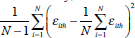 , where ε is the forecast error.
Other definitions of forecast disagreement also exist. See, for example,
Dovern et al (2009).
[25]
, where ε is the forecast error.
Other definitions of forecast disagreement also exist. See, for example,
Dovern et al (2009).
[25]
This explains why levels cease changing in the last few years of the sample. It was thought to be preferable to show the results in this manner rather than, say, reduce the span of the sample over which d was estimated. [26]
There are other panel unit root tests that have been shown to be more powerful in a statistical sense. Siklos (2009b) and references therein consider some of these. Given the results reported below, it is unlikely that the conclusions will be much changed. Moreover, the extant literature is more familiar with the tests reported here. [27]
LLC advocate removing the overall mean of the series (that is,  ) prior to running the test. It is not immediately
obvious that this is necessary when the series under investigation is a differential
between two existing series.
[28]
) prior to running the test. It is not immediately
obvious that this is necessary when the series under investigation is a differential
between two existing series.
[28]
Enders and Siklos (2001) propose a strategy to test for threshold cointegration. The test relies on the ADF form for the test equation where the error correction term is replaced with two error corrections terms that switch depending on whether the series in question is above or below some estimated threshold, resulting in the threshold autoregressive (TAR) formulation. For reasons having to do with the statistical power of such tests, the so-called momentum TAR (M-TAR) is preferred. In this version, it is the change in the error correction term vis-à-vis some threshold that switches from a positive to a negative state that adds asymmetry to the conventional ADF-type specification. [29]
For Australia, a total of 7 forecasts were retained. For the other countries the numbers are provided in parentheses: Canada (7), New Zealand (8), Sweden (11), the United Kingdom (10), euro area (11), Japan (8), Switzerland (5) and the United States (11). [30]
Space constraints prevent a full discussion. However, the object of the exercise is to find the highest eigenvalues from the eigenvectors estimated from the covariance matrix that describes the relationship between the series of interest. Additional details can be found in, among other sources, Maddala (1977, pp 193–194) and Jolliffe (1986). [31]
An alternative approach, currently the subject of ongoing work, consists of estimating a version of Equation (3) via quantile regressions in order to better exploit the information contained in the distribution of forecasts. [32]
A Hausman test (results not shown) does suggest that the full-sample model may be mis-specified. What is unclear is the form of the mis-specification. It could be that the null that κ is constant across cross-sections is incorrect or it could be the case that it is inappropriate to pool all the economies in our sample together. For example, one might consider a separate pool of IT economies and non-IT economies. This extension is left for future research. [33]
Using rates of change in these series does not appear to make much difference. However, in line with the earlier discussion, it seems preferable to think in terms of a measure of disequilibrium in relative prices. Needless to say, there are well-known drawbacks in using the HP filter but it is so widely applied that whatever it loses in terms of precision, it makes up for by remaining comparable with the relevant literature. The default smoothing parameter of 1,600 is used in all HP-filtered estimates. [34]
The variance of fd was also considered but was generally found to be statistically insignificant. Hence, it was omitted from the final specification. [35]
All specifications include fixed effects At and this version of Equation (3) could not be rejected. [36]
The somewhat arbitrary choice of sub-samples does not address the question of whether the reduction in inflation persistence was achieved faster in IT or non-IT economies, nor is the precise year when persistence became statistically significant identified for each economy. [37]
References
Acemoglu D, S Johnson, P Querubín and JA Robinson (2008), ‘When Does Policy Reform Work? The Case of Central Bank Independence’, Brookings Papers on Economic Activity, 1, pp 351–417.
Baillie RT, C-F Chung and MA Tieslau (1996), ‘Analyzing Inflation by the Fractionally Integrated ARFIMA-GARCH Model’, Journal of Applied Econometrics, 11(1), pp 23–40.
Ball LM (2006), ‘Has Globalization Changed Inflation?’, NBER Working Paper No 12687.
Benati L (2008), ‘Investigating Inflation Persistence across Monetary Regimes’, Quarterly Journal of Economics, 123(3), pp 1005–1060.
Bernanke BS (2007), ‘Inflation Expectations and Inflation Forecasting’, speech given at the Monetary Economics Workshop Summer Institute of the National Bureau of Economic Research, Cambridge, 10 July.
Bernanke BS (2008), ‘Outstanding Issues in the Analysis of Inflation’, speech given at the Federal Reserve Bank of Boston's 53rd Annual Economic Conference, Chatham, 9 June.
Bernanke BS, T Laubach, FS Mishkin and AS Posen (1999), Inflation Targeting: Lessons from the International Experience, Princeton University Press, Princeton.
Bertrand M, E Duflo, and S Mullainathan (2004), ‘How Much Should We Trust Differences-In-Differences Estimates?’, Quarterly Journal of Economics, 119(1), pp 249–275.
Blinder AS (1999), Central Banking in Theory and Practice, MIT Press, Cambridge.
Blinder AS, M Ehrmann, M Fratzscher, J De Haan and D-J Jansen (2008), ‘Central Bank Communication and Monetary Policy: A Survey of Theory and Evidence’, Journal of Economic Literature, 46(4), pp 910–945.
Bohl MT, DG Mayes and PL Siklos (forthcoming), ‘The Quality of Monetary Policy and Inflation Performance: Globalization and Its Aftermath’, The Manchester School.
Borio C and P Lowe (2004), ‘Securing Sustainable Price Stability: Should Credit Come Back from the Wilderness?’, BIS Working Paper No 157.
Borio C and A Filardo (2007), ‘Globalisation and Inflation: New Cross-Country Evidence on the Global Determinants of Domestic Inflation’, BIS Working Paper No 227.
Carlson JA and M Parkin (1975), ‘Inflation Expectations’, Economica, 4(166), pp 123–138.
Cecchetti SG, P Hooper, BC Kasman, KL Schoenholtz and MW Watson (2007), ‘Understanding the Evolving Inflation Process’, report presented at the 2007 Meeting of the U.S. Monetary Policy Forum, Washington DC, 9 March. Available at <http://www.princeton.edu/~mwatson/papers/USMPF_Report_July_2007.pdf>.
Côté D and C de Resende (2008), ‘Globalization and Inflation: The Role of China’, Bank of Canada Working Paper No 2008-35.
Dovern J, U Fritsche, and J Slacalek (2009), ‘Disagreement among Forecasters in G7 Countries’, ECB Working Paper No 1082.
Enders W (2004), Applied Time Series Analysis, 2nd edn, John Wiley & Sons, New York.
Enders W and PL Siklos (2001), ‘Cointegration and Threshold Adjustment’, Journal of Business and Economic Statistics, 19(2), pp 166–176.
Gagnon JE and J Ihrig (2004), ‘Monetary Policy and Exchange Rate Pass-Through’, International Journal of Finance & Economics, 9(4), pp 315–338.
Hamilton JD (2009), ‘Causes and Consequences of the Oil Shock of 2007–08’, Brookings Papers on Economic Activity, 1, pp 215–261.
Hassler U and J Wolters (1995), ‘Long Memory in Inflation Rates: International Evidence’, Journal of Business and Economic Statistics, 13(1), pp 37–45.
Hooker MA (2002), ‘Are Oil Shocks Inflationary? Asymmetric and Nonlinear Specifications versus Changes in Regime’, Journal of Money, Credit and Banking, 34(2), pp 540–561.
Ihrig J, SB Kamin, D Lindner and J Marquez (2007), ‘Some Simple Tests of the Globalization and Inflation Hypothesis’, Board of Governors of the Federal Reserve System International Finance Discussion Paper No 891.
Im KS, MH Pesaran and Y Shin (2003), ‘Testing for Unit Roots in Heterogenous Panels’, Journal of Econometrics, 115(1), pp 53–74.
Jolliffe IT (1986), Principal Component Analysis, Springer-Verlag, New York.
Kiley MT (2008), ‘Monetary Policy Actions and Long-Run Inflation Expectations’, Board of Governors of the Federal Reserve System Finance and Economics Discussion Series No 2008-03.
Lahiri K and X Sheng (2008), ‘Measuring Forecast Uncertainty by Disagreement: The Missing Link’, Ifo Working Paper No 60.
Levin A, C-F Lin and C-SJ Chu (2002), ‘Unit Root Tests in Panel Data: Asymptotic and Finite Sample Properties’, Journal of Econometrics, 108(1), pp 1–24.
Maddala GS (1977), Econometrics, McGraw-Hill, New York.
Mankiw NG, R Reis and J Wolfers (2004), ‘Disagreement about Inflation Expectations’, in M Gertler and KS Rogoff (eds), NBER Macroeconomic Annual 2003, 18, MIT Press, Cambridge, pp 209–248.
Mishkin FS (2007a), ‘Headline versus Core Inflation in the Conduct of Monetary Policy’, speech presented at the ‘Business Cycles, International Transmission and Macroeconomic Policies’ Conference, HEC Montréal, Montreal, 20 October.
Mishkin FS (2007b), Monetary Policy Strategy, MIT Press, Cambridge.
Orphanides A and JC Williams (2007), ‘Robust Monetary Policy with Imperfect Knowledge’, Journal of Monetary Economics, 54(5), pp 1406–1435.
Pesaran MH (1985), ‘Formation of Inflation Expectations in British Manufacturing Industries’, Economic Journal, 95(380), pp 948–975.
Pesaran MH (1987), The Limits to Rational Expectations, Basil Blackwell, Oxford.
Reis R and MW Watson (2009), ‘Relative Goods' Prices, Pure Inflation, and the Phillips Correlation’, working paper, Princeton University, January.
Rogoff KS (2003), ‘Globalization and Global Disinflation’, in Monetary Policy and Uncertainty: Adapting to a Changing Economy, a Symposium sponsored by the Federal Reserve Bank of Kansas City, Jackson Hole, pp 77–112.
Rose AK (2007), ‘A Stable International Monetary System Emerges: Inflation Targeting is Bretton Wood, Reversed’, Journal of International Money and Finance, 26(5), pp 663–681.
Rudd J and K Whelan (2007), ‘Modeling Inflation Dynamics: A Critical Review of Recent Research’, Journal of Money, Credit and Banking, 39(s1), pp 155–170.
Sargent TJ (1999), The Conquest of American Inflation, Princeton University Press, Princeton.
Shiller RJ (1997), ‘Why Do People Dislike Inflation?’, in CD Romer and DH Romer (eds), Reducing Inflation: Motivation and Strategy, University of Chicago Press, Chicago, pp 13–65.
Siklos PL (1999a), ‘Inflation-Target Design: Changing Inflation Performance and Persistence in Industrial Countries’, Federal Reserve Bank of St. Louis Review, 81(2), pp 47–58.
Siklos PL (1999b), ‘Pitfalls and Opportunities for the Conduct of Monetary Policy in a World of High-Frequency Data’, in Information in Financial Asset Prices, Proceedings of a Conference, Bank of Canada, Ottawa, pp 331–369.
Siklos PL (2002), The Changing Face of Central Banking: Evolutionary Trends since World War II, Cambridge University Press, Cambridge.
Siklos PL (2009a), ‘As Good as It Gets? The International Dimension to Canada's Monetary Policy Strategy Choices’, C.D. Howe Institute Commentary, No 292. Available at <http://www.cdhowe.org/pdf/commentary_292.pdf>.
Siklos PL (2009b), ‘Meeting Maastricht: Nominal Convergence of the New Member States toward EMU’, Wilfrid Laurier University, Department of Economics Working Paper, August.
Smith J and M McAleer (1995), ‘Alternative Procedures for Converting Qualitative Response Data to Quantitative Expectations: An Application to Australian Manufacturing’, Journal of Applied Econometrics, 10(2), pp 165–185.
Stock JH and MW Watson (2007), ‘Why Has U.S. Inflation Become Harder to Forecast?’, Journal of Money, Credit and Banking, 39(s1), pp 3–33.
Tay AS and KF Wallis (2000), ‘Density Forecasting: A Survey’, Journal of Forecasting, 19(4), pp 235–254.
Taylor JB (2010), ‘Globalization and Monetary Policy: Missions Impossible’, in J Galí and M Gertler (eds), International Dimensions of Monetary Policy, University of Chicago Press, Chicago, pp 609–624.
Trichet J-C (2009), ‘Credible Alertness Revisited’, intervention at the Symposium on ‘Financial Stability and Macroeconomic Policy’ sponsored by the Federal Reserve Bank of Kansas City, Jackson Hole, 22 August.
Warren GF and FA Pearson (1932), Wholesale Prices for 213 Years, 1720 to 1932: Part I, Memoir 142, Cornell University Agricultural Experiment Station, Ithaca.