RBA Annual Conference – 2009 Measuring Core Inflation in Australia with Disaggregate Ensembles Francesco Ravazzolo and Shaun P Vahey^[1]

1. Introduction

Since the introduction of inflation targeting, many central banks have focused greater attention on the behaviour of measured inflation. Unfortunately, the theoretical concept of inflation is conceptually mismatched with the headline consumer price index (CPI) measure; see, for example, the arguments in Quah and Vahey (2005). In particular, relative price movements are confounded with general price movements. For example, should we think of recent increases in commodity prices as part of inflation or as movements in relative prices?

A number of central banks regularly examine disaggregate inflation series for less volatile and leading evidence of the inflationary process. The aim in using a ‘core’ or ‘underlying’ measure to communicate inflationary pressures is that the influence of relative prices can be removed, or at least moderated. (Hereafter, we use the terms core and underlying interchangeably.) One popular approach truncates (and averages) the disaggregate inflation (or price) cross-sectional distribution to provide a ‘core’ measure. A second approach excludes particular disaggregates, that is, they receive zero weight; the resulting measure is commonly referred to as an ‘ex’ core measure. In practice, which series are discarded varies across central banks and through time. Although theoretical considerations are often advanced as a justification for both of these approaches, there is considerable uncertainty over which disaggregates or what proportion of the cross-section should be discarded.

Faced with these and other ambiguities in defining core inflation, practitioners often evaluate candidate core inflation measures based on forecasting performance; see, for example, Roger (1998), Wynne (1999) and Smith (2004). The jury is still out on whether core measures offer any advantage over a simple autoregressive benchmark for measured inflation in terms of the out-of-sample accuracy of point forecasts.

In this paper, we reformulate the measuring underlying inflation issue. We start by focusing directly on the forecasting problem, limiting our attention to candidate disaggregate series as forecasting variables. In contrast to the earlier literature on core inflation, we assess forecasting performance based on the complete density for inflation. Tests of point forecast accuracy provide no guidance on the usefulness of core measures for general (but unknown) loss functions.

Our ensemble methodology follows the analysis of inflation in the United States by Ravazzolo and Vahey (2009). We construct ensemble predictive densities based on the out-of-sample forecast performance of many component models, where each model uses a particular disaggregate series. This approach provides well-calibrated forecast densities for measured inflation in Australia. Combining the evidence from two sources of disaggregation, by city and by sector, yields considerable improvement in density performance. The resulting forecast densities are preferable to those from a benchmark autoregressive model, with competitive point forecast performance. The traditional weighted median and trimmed mean measures of core inflation sometimes differ considerably from the median of the forecast density. For example, the probability of inflation being overstated by the (subsequently published) trimmed mean measure was more than 75 per cent for 2008:Q1.

In our application, we focus entirely on one-quarter-ahead forecasts. Within the underlying inflation literature, the horizon of interest varies, typically between one and eight quarters ahead. Although longer horizon ensemble forecasts are possible with our methodology, we concentrate on horizons much shorter than typically focused on by many inflation-targeting central banks. Our hope is that the disaggregate ensemble core measure picks up the inflation already in the pricing pipeline, and does not respond to future changes in policy stance. For further discussion of the choice of forecasting horizon in the core inflation literature, see Brischetto and Richards (2006).

The remainder of this paper is as follows. We provide a brief review of the core inflation literature in Section 2. The ensemble modelling strategy is discussed in Section 3. We describe our component models and our ensemble predictives in Section 4. The Australian dataset is summarised in Section 5, and results are presented in Section 6. Some conclusions are drawn in Section 7.

2. A Brief Review of the Core Inflation Literature

It is widely recognised by the public and central bankers that movements in the CPI do not always capture true ‘inflationary’ pressures. The weights on the disaggregates in the cost of living index reflect the preferences and budget constraint of the representative consumer. But those weights can lead to a misleading assessment of inflationary pressures because relative price changes are confounded with sustained general price movements.

In the core inflation literature, the aim is to measure the general increase in prices. Most central banks consider a variety of measures of underlying inflation. Many of these are derived by removing an ‘unwanted’ component, which is often treated as ‘noise’; for further discussion see Brischetto and Richards (2006).

Traditional methods for measuring core inflation include smoothing and structural time-series modelling. The first of these takes a moving average of measured inflation and labels this as the core. The second makes specific assumptions about the functional form for underlying inflation (such as taking it to be a Gaussian random walk) and produces an estimate with the Kalman filter.

Partly as a result of dissatisfaction with the ability of these models to forecast inflation, many central banks consider measures of core inflation obtained by applying zero weights to particular components. Bryan and Cecchetti (1994) extend this exclusion-based methodology by zero-weighting the disaggregates in the tails of the cross-section. Although Bryan and Cecchetti offer a menu cost model as a rationale for truncating the distribution, that theory does not imply any particular truncation factor for the disaggregate distribution.

A related problem blights the less complex ‘ex’ core measures that always exclude particular components. The argument for using ‘ex’ measures is that: if you know that one or two (or more) disaggregate series contain a great deal of ‘noise’, then they should be dropped from measured inflation to form the core measure. This is the argument, for example, regarding the personal consumption expenditures chain-type price index excluding food and energy in the United States (Ravazzolo and Vahey 2009).

Unfortunately, zero-weighting disaggregate components rarely produces a core measure that beats simple autoregressive benchmarks in out-of-sample forecast evaluations. Moreover, the uncertainties involved in the selection of truncation factors, or the series to be excluded, affect the usefulness of the candidate core measures as communication tools. The public often suspect that the central bank exploiting these communication devices prefers to ignore inconvenient data. For example, the December 1997 Reserve Bank of New Zealand background briefing for the Policy Targets Agreement explicitly draws attention to this difficulty.^[2]

In our ensemble approach described below, we avoid using strong off-model or prior information about which disaggregates are likely to provide useful signals regarding future values of measured inflation. Instead, we formulate the problem of measuring core inflation as one of combining component forecast densities of measured inflation, where each component is based on a particular disaggregate series. In this sense, we let the data speak clearly about which disaggregates are important for density forecasts of measured inflation. If particular disaggregates do not matter for inflation in the next quarter, they receive a small weight (bounded at zero). In so doing, we formally account for the uncertainty regarding which disaggregates should be included, and also over the type of disaggregation.

3. Modelling Strategy

Garratt, Mitchell and Vahey (2009) drew attention to the antecedents of ensemble macro modelling in statistics and weather forecasting. Outside of the econometrics literature, the benefits of the ensemble approach to forecasting have been recognised for around 15 years. Meteorologists and statisticians have focused a great deal of attention on analysing statistical ensembles. The idea behind the ensemble approach is to consider a large number of models, each of which is a variant or component of the ‘preferred’ specification. Each component could be viewed as an approximation of the current state of the ‘true’ but unknown specification, and when considered together, the ensemble approximates the truth.

In the meteorological forecasting literature, the ensemble methodology is a response to what macro-econometricians sometimes call ‘uncertain instabilities’ (see Clark and McCracken 2007, for example). Individual empirical specifications tend to exhibit instabilities, which can be difficult to isolate with short runs of real-time macroeconomic data.

Bache et al (2009) list four common characteristics of an ensemble strategy for macro modelling:

1. generation of forecasting densities, rather than point forecasts;
2. predictive density construction from a large number of component macroeconometric models;
3. forecast density evaluation and combination based on out-of-sample performance, rather than in-sample analysis; and
4. component model weights vary through evaluation – ensemble densities have time-varying weights.

Papers in the economics literature that satisfy these criteria include: Jore, Mitchell and Vahey (2008), Garratt et al (2009) and Kascha and Ravazzolo (2010). Smith et al (2009) consider the performance of the Norges Bank ‘nowcasting’ system, which also adopts the ensemble methodology. In these cases, the out-of-sample densities from many macroeconometric component models are directly combined into the ensemble using an ‘opinion pool’.^[3] These papers differ in the design of the model space and the number of components considered, as well as the applied problem of interest.

Another strand of the economics literature uses informative priors for the combination step to produce ensembles. Maheu and Gordon (2008) and Geweke (2010) use mixture models to give non-Gaussian predictives. Andersson and Karlsson (2007) take a predictive likelihood approach to combining vector autoregressions (VARs).

Geweke (2010) discusses the relationships between density pooling and mixture modelling, and argues that the former presents a more coherent approach for incomplete model spaces. Clearly, both variants can be effective methods for combining densities in forecasting applications. In a related literature, Patton (2004), Maheu and McCurdy (2009) and Amisano and Geweke (2010) consider ensembles in various financial applications.

Before we move on to discuss the model space and ensembles for our application, it is worth considering whether we want to forecast the entire density of measured inflation. In our view, restricting attention to point forecast accuracy makes no sense. There is no reason to believe that the inflation process is Gaussian; and there is nothing particularly compelling about the quadratic loss function. In the absence of either assumption, the root mean squared forecast error (RMSFE) metric has no justification. If we want to forecast inflation, the whole forecast density seems a natural starting point.

4. Component Model Space and Ensembles

For each observation in the policy-maker's out-of-sample ‘evaluation period’, we use density forecast performance to compute the weight on each component model. The component models use a common time-series structure, namely an autoregressive specification with four lags, AR(4).^[4] Each component model uses a particular disaggregate inflation measure. The weights on the individual components are based on the ‘fit’ of the component predictive densities for measured inflation. Given these weights, we construct ensemble forecast densities for measured inflation.

More formally, consider a policy-maker aggregating N forecasts from different ‘sources’, each using a unique component forecasting model. Given i = 1, …, N components (where N could be a large number), we define the ensemble measure of core inflation by the convex combination also known as a linear opinion pool:

where are the h-step-ahead forecast densities from component model i, i = 1, …, N, conditional on the information set I_τ.

Each component model forecasts disaggregate inflation. Then in each recursion, we centre the component forecasts on measured inflation. In effect, this step restricts the ensemble forecast density to be uni-modal but not symmetric. Bao et al (2007) discuss the common practice of centring ensemble forecast densities prior to combination.

After this centring procedure, each component model produces h-step-ahead forecast densities for measured inflation, g(•). Each component model uses data, dated τ – h or earlier, to produce a h-step-ahead forecast density for τ. The non-negative weights, w_i,τ,h, in this finite mixture sum to unity, are positive, and vary by recursion in the evaluation period .

We emphasise that the ensemble forecast density has the scope to be non-Gaussian even if the component models produce Gaussian predictives. The linear opinion pool ensemble (Equation (1)) accommodates skewness and kurtosis. The flexible structure resulting from linear pooling allows the data to reveal whether, for example, the ensemble should have fat tails, or asymmetries.^[5]

We construct the ensemble forecast density for measured inflation using Equation (1). Implementation of the density combination requires a measure of component density fit to provide the weights. A number of recent applications in the economics literature have used density scoring rules. In this application, we utilise the continuous ranked probability score (CRPS), which as (among others) Gneiting and Raftery (2007), Panagiotelis and Smith (2008) and Ravazzolo and Vahey (2009) note, rewards predictive densities from components with high probabilities near (and at) the actual outcome.^[6]

The weights for the h-step-ahead disaggregate ensemble (DE) CPI densities are:

where is the centred predictive density for measured aggregate inflation π_τ,h given by model i; and X is the CRPS-based measure of density performance as in Ravazzolo and Vahey (2009).

Using Equations (1) and (2), we construct two disaggregate ensembles that combine predictive densities from cities, and sectors, respectively. The city DE, denoted DE_c, contains eight components (city disaggregates); the sector DE, DE_s, contains 10 components (sector disaggregates). We also use the ‘grand ensemble’ technique proposed by Garratt et al (2009) to combine the two ensembles based on different types of disaggregation. Given the short sample in our application, we give equal weight to the ensembles, DE_c and DE_s in constructing the grand ensemble, denoted, DE_cs.^[7]

As a benchmark for our forecast evaluations, we use an AR(4) model for measured inflation. (We experimented with various lag orders for the benchmark and found the results to be qualitatively similar.) Our choice of an autoregressive benchmark was motivated by the Stock-Watson observation that similar specifications are ‘hard to beat’ in out-of-sample forecast evaluations. We use non-informative priors for the AR(4) parameters, with an expanding window for estimation – so that forecasts are recursive. The predictive densities follow the t-distribution, with mean and variance equal to OLS estimates (see Koop 2003 for details).

To assess the calibration properties of the ensemble densities we follow Diebold, Gunther and Tay (1998) and compute probability integral transforms, PITS. We apply the Berkowitz (2001) likelihood ratio test for independence, zero mean and unit variance of the PITS. The test statistic is distributed χ² (3) under the null hypothesis of no calibration failure, with a maintained hypothesis of normality. We also report the average (over the evaluation period ) logarithmic score. The logarithmic score of the i-th density forecast, ln , is the logarithm of the probability density function , evaluated at the outcome π_τ,h. Hence, the log score evaluates the predictives at the outcome only. We investigate relative predictive accuracy by considering a test based on the Kullback-Leibler information criterion (KLIC), derived from the expected difference in the log scores of the two models; see Mitchell and Hall (2005), Amisano and Giacomini (2007) and Bao, Lee and Saltoglu (2007). Suppose that there are two ensemble forecast densities, and , so that the KLIC differential between them is the expected difference in their log scores: . The null hypothesis of equal density forecast accuracy is H₀ : E(d_τ,h)=0. A test can then be constructed since the mean of d_τ,h over the evaluation period, d_τ,h, under appropriate assumptions, has the limiting distribution: , where Ω is a consistent estimator of the asymptotic variance of d_τ,h.^[8] Mitchell and Wallis (2008) explain the importance and practical difficulties of using information-based methods to discriminate between competing forecast densities.

5. Data

We apply our ensemble methodology to combine Australian disaggregate inflation forecasts for quarter-on-quarter growth of the CPI. We assess the performance of the disaggregate ensembles, and other core measures, using an evaluation period from 1997:Q1 to 2008:Q4 (48 observations). The period 1994:Q4 to 1996:Q4 is used as a ‘training period’ to initialise the ensemble weights.^[9]

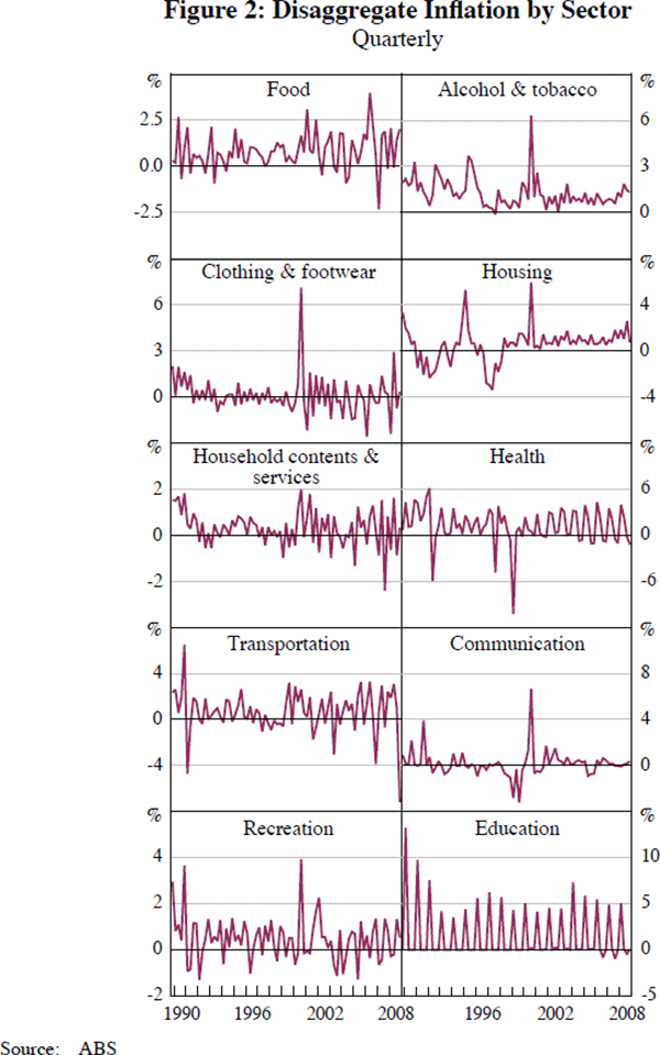
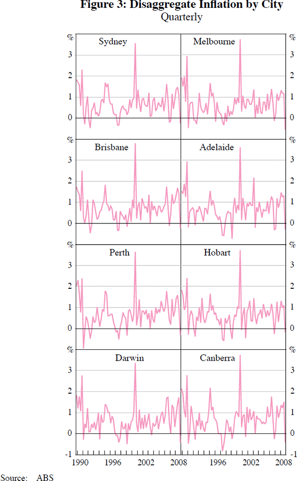
As mentioned above, the Australian CPI can be broken down by sectors and cities. The first breakdown decomposes the CPI into 10 disaggregates representing sectors. In our empirical analysis, we exclude the sector ‘financial and insurance services’ for which there are data from 2005:Q3 only. The second form of disaggregation decomposes the CPI according to data on prices from eight cities.

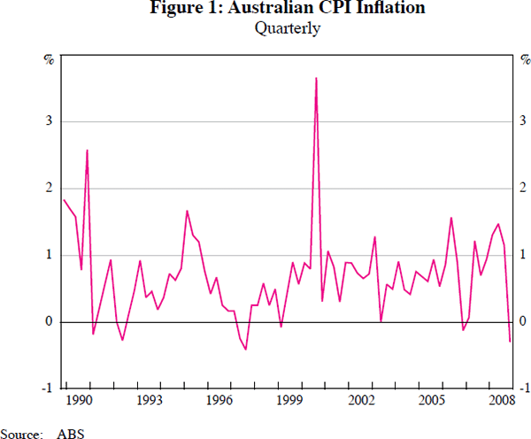
Figures 1, 2 and 3 plot respectively the CPI, its sector disaggregates and its city disaggregates over the sample 1989:Q4–2008:Q4. One striking feature is the high degree of contemporaneous dependence across cities. In contrast, the sectors display more heterogeneity, with differences in means and volatility.

6. Results

Recall that we construct the core inflation measure, DE, by combining the predictive densities from the disaggregate component models. We compare and contrast the ensembles using disaggregation by sector DE_s, by city DE_c, and the grand ensemble of the two, DE_cs. Below we report evaluations for the one-step-(one-quarter-) ahead horizon.^[10]

Before turning to the density evaluations for our various ensembles, we summarise point forecast performance. The RMSFE of DE_s, DE_c, DE_cs, and the benchmark AR(4) are 0.558, 0.424, 0.473 and 0.378, respectively. The Clark and West (2006) test for superior predictive accuracy (against the null of equal accuracy) indicates that the ensembles are competitive with the AR(4) benchmark with test statistics of 1.592, 1.556, 1.574 for the DE_s, DE_c, and DE_cs, respectively. The critical value for rejection of the null for a 95 per cent interval is 1.645. Smith (2004) and Kiley (2008) discuss the properties of various point forecasts for core inflation measures. Most fail to outperform simple autoregressive benchmarks.

We turn now to the ex post (end of period) evaluation of the forecast densities from the ensemble forecasts and the benchmark. Table 1 has four rows; one for each ensemble and the benchmark. The columns report (reading from left to right) the Berkowitz likelihood ratio test (based on the PITS), the log scores (averaged over the evaluation period) and the p-values for the equal predictive density accuracy test (based on the log scores), respectively. Whereas DE_s, DE_c and DE_cs appear to be well-calibrated on the basis of the Berkowitz likelihood ratio, the final column shows that the AR(4)is rejected in favour of DE_cs only in the case of the KLIC-based test. The ensemble DE_cs delivers a statistically significant improvement in the log score (reported in the second column) based on a 95 per cent confidence interval.

Table 1: Forecast Performance

	LR	LS	LS-test
AR(4)	0.185	−1.078
DE_s	0.222	−0.940	0.148
DE_c	0.184	−1.062	0.383
DE_cs	0.215	−0.864	0.037
Notes: The column LR is the likelihood ratio p-value of the test of zero mean, unit variance and independence of the inverse normal cumulative distribution function-transformed PITS, with a maintained assumption of normality for transformed PITS. LS is the average logarithmic score, averaged over the evaluation period. LS-test is the p-value of the KLIC-based test for equal density forecasting performance of AR(4) and DE12 over the sample 1997:Q1 to 2008:Q4.

The weights in DE_s and DE_c display some variation through time. Tables 2 and 3 report the weights on the sector and city disaggregates, respectively, for three specific observations. It can be seen from both tables that generally all disaggregate components have a non-zero weight. There does not seem to be a case for excluding the information on individual disaggregates, or groups of particular disaggregates, on the basis of these weights.^[11]

Table 2: Disaggregate Weights – DE_s

	1997:Q1	2002:Q4	2008:Q4
Food	0.166	0.178	0.156
Alcohol & tobacco	0.100	0.098	0.110
Clothing & footwear	0.095	0.068	0.080
Housing	0.077	0.086	0.100
Household contents & services	0.150	0.159	0.128
Health	0.066	0.068	0.070
Transportation	0.094	0.112	0.104
Communication	0.122	0.095	0.111
Recreation	0.085	0.093	0.101
Education	0.046	0.044	0.041

Table 3: Disaggregate Weights – DE_c

	1997:Q1	2002:Q4	2008:Q4
Sydney	0.087	0.073	0.084
Melbourne	0.123	0.150	0.146
Brisbane	0.138	0.126	0.116
Adelaide	0.098	0.122	0.117
Perth	0.076	0.117	0.110
Hobart	0.110	0.142	0.157
Darwin	0.205	0.138	0.137
Canberra	0.162	0.132	0.133

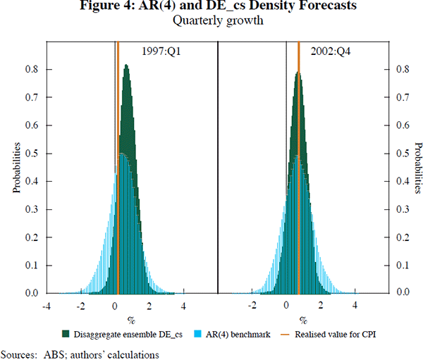
To provide insight into the probability of inflation events, Figure 4 provides the ensemble forecast densities from DE_cs at particular observations, namely 1997:Q1 and 2002:Q4 (the first and the middle observations in our evaluation period), together with the benchmark densities. We see that the AR(4) benchmark produces density forecasts that are too wide, with a high probability mass attributed to (quarterly) inflation in excess of 2 per cent in absolute value for both observations. The core predictives contain more mass in the regions around the actual outcomes than the AR(4) benchmark, with minor departures from symmetry.

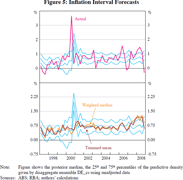
Returning to the issue of measuring core inflation, recall that, in this paper, we reformulate the problem of measuring underlying inflation. We focus on constructing complete forecast densities for measured inflation and limit our set of candidate forecasting variables to disaggregate series. We describe our disaggregate ensemble forecast density for measured inflation as the measure of core inflation. How should we interpret the traditional weighted median and trimmed mean measures of core inflation conditional on our density forecast? In Figure 5, we plot the median from our grand ensemble core, DE_cs, together with the 25th and 75th percentiles, through the evaluation period. The DE_cs core ignores several extreme values in the actual measured inflation series – the forecast median of this measure is fairly smooth.^[12] This figure also plots the trimmed mean and weighted median measures of core inflation used by the Reserve Bank of Australia; see Appendix A for details. The DE core inflation measure suggests that both of these periodically give assessments of inflationary pressures that are low-probability. The year 2008 saw several outcomes above the 75th percentile for both of these underlying measures. The DE core implies that inflationary pressures were more moderate. For example, according to the DE core measure, the probability of inflation being overstated by the trimmed mean measure was more than 75 per cent for 2008:Q1. We should note also that the traditional measures of underlying inflation plotted here are less timely than the DE core, which is a well-calibrated one-step-ahead forecast density.

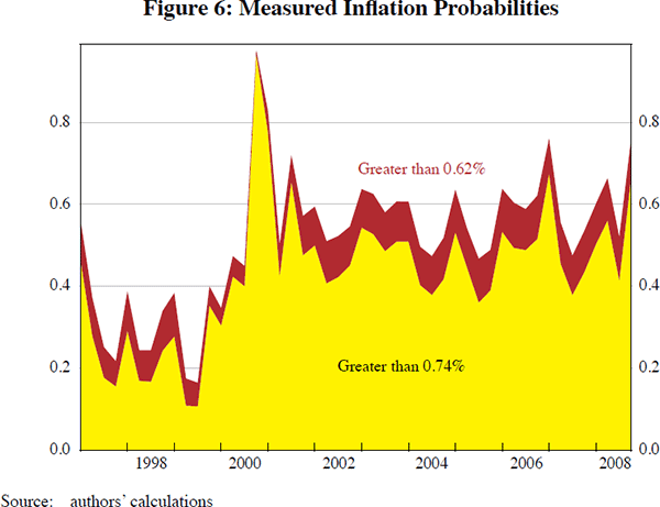
One advantage of our probabilistic approach to measuring core inflation is that we can calculate the probability of specific events for measured inflation of interest to policy-makers. As an example, we calculate the (one-step-ahead) probability that measured inflation exceeds the upper range and midpoint of the inflation target. The target for monetary policy in Australia is to achieve an inflation rate of 2–3 per cent, on average, over the cycle (in annualised terms). We work with analogous thresholds for the one-step-ahead horizon, interpreted at a quarterly frequency. The events of interest are: (1) measured inflation greater than 0.74 per cent (upper range of the target); and (2) measured inflation greater than 0.62 per cent (midpoint of the target). The time series for the probabilities of these two events are plotted in Figure 6. As a visual aid, we label the ‘upper range’ event yellow, and the ‘midpoint’ event red, and shade the plot appropriately. The figure suggests that the probability of exceeding the upper threshold has generally been around 50 per cent in recent years. The probability of measured inflation exceeding the midpoint of the band is typically greater than 50 per cent.

7. Conclusions

Instead of gauging core inflation by traditional methods, we have focused on the problem of constructing an ensemble forecast density. We conclude from our analysis that the ensemble approach provides well-calibrated forecast densities for Australian measured inflation from disaggregate information. Our forecast densities use information from disaggregation both by city and by sector, and indicate that more traditional core measures at times fail to strip out the impact of relative prices in measured inflation.

Appendix A: Traditional Core Measures

Extract from ‘Notes to Tables’, Reserve Bank of Australia Bulletin, December 2009 (Table G.1 Measures of Consumer Price Inflation, pp S118–S119):

The ‘Weighted median’ and ‘Trimmed mean’ are calculated using the component level data of the consumer price index. Both measures exclude interest charges prior to the September quarter 1998 and are adjusted for the tax changes of 1999–2000. The ‘Trimmed mean’ is calculated by ordering all the CPI components by their price change in the quarter and taking the expenditure-weighted average of the middle 70 per cent of these price changes. The ‘Weighted median’ is the price change in the middle of this ordered distribution, taking also expenditure weights into account. Annual rates of ‘Weighted median’ and ‘Trimmed mean’ inflation are calculated based on compounded quarterly rates. For calculating the ‘Weighted median’ and ‘Trimmed mean’, where CPI components are identified as having a seasonal pattern, quarterly price changes are estimated on a seasonally adjusted basis. Seasonal adjustment factors are calculated as concurrent factors, that is using the history of price changes up to and including the current CPI release. There is a series break at September 2002 due to the ABS publishing the ‘Weighted median’ and ‘Trimmed mean’ on behalf of the RBA from that point forward, using data to a higher level of precision than is publicly available.

For further information on the various measures of underlying consumer price inflation, refer to ‘Box D: Underlying Inflation’, Statement on Monetary Policy, May 2002; ‘Box D: Measures of Underlying Inflation’, Statement on Monetary Policy, August 2005; and Roberts (2005), ‘Underlying Inflation: Concepts, Measurement and Performance’, Reserve Bank of Australia Research Discussion Paper No 2005-05.

Footnotes

F Ravazzolo: Norges Bank, Research Department; email: francesco.ravazzolo@norges-bank.no. S Vahey: University of Melbourne; email: spvahey@gmail.com.

We thank the editors, Renée Fry, Callum Jones and Christopher Kent, as well as conference participants for comments. In particular, we are grateful to our discussant Tony Richards for helpful advice. [1]

See <http://www.rbnz.govt.nz/monpol/pta/0055243.html>. [2]

Wallis (2005) uses opinion pools to average (model free) survey forecasts, rather than those from macroeconometric models. Mitchell and Hall (2005) use opinion pools to combine forecasts from two institutions. Gerard and Nimark (2008) consider opinion pool combinations with three macro models. [3]

Ravazzolo and Vahey (2009) consider time-varying parameter components but find that simple autoregressive components result in a relatively small drop in forecast performance. [4]

Kascha and Ravazzolo (2010) compare and contrast logarithmic and linear pooling. Logarithmic opinion pools force the ensemble predictives to be symmetric, but accommodate fat tails; see also Smith et al (2009). [5]

See Panagiotelis and Smith (2008) for an explanation of how CRPS is calculated in practice. [6]

Garratt et al (2009) explore the use of recursively estimated weights to construct their grand ensembles. [7]

When evaluating the ensemble forecast densities we treat them as primitives, and abstract from the ensemble combination methodology. Giacomini and White (2006) and Amisano and Giacomini (2007) discuss more generally the limiting distribution of related test statistics. [8]

Data are available from the Australian Bureau of Statistics at <http://www.abs.gov.au> (ABS Cat No 6401.0). [9]

We also computed, but do not report, forecasts for two-, three- and four-step-ahead horizons. Results are qualitatively similar and available upon request from the authors. [10]

Geweke (2010) argues that even a zero weight is not sufficient to conclude that a component model has zero value for the linear opinion pool. [11]

Following the suggestion of our discussant, we also experimented with a CPI series, and disaggregate series, with tax effects removed. For most of the evaluation period, the forecast densities for measured inflation were almost identical to those reported in this paper. The exception is the spike at the start of this decade, which does not appear in the forecasts with tax-adjusted data. [12]

References

Amisano G and J Geweke (2010), ‘Comparing and Evaluating Bayesian Predictive Distributions of Asset Returns’, International Journal of Forecasting, 26(2), pp 216–230.

Amisano G and R Giacomini (2007), ‘Comparing Density Forecasts via Weighted Likelihood Ratio Tests’, Journal of Business & Economic Statistics, 25(2), pp 177–190.

Andersson MK and S Karlsson (2007), ‘Bayesian Forecast Combination for VAR Models’, Sveriges Riksbank Working Paper No 216.

Bache IW, J Mitchell, F Ravazzolo and SP Vahey (2009), ‘Macro Modelling with Many Models’, National Institute of Economic and Social Research Discussion Paper No 337.

Bao L, T Gneiting, EP Grimit, P Guttop and AE Raftery (2007), ‘Bias Correction and Bayesian Model Averaging for Ensemble Forecasts of Surface Wind Direction’, University of Washington, Department of Statistics, Technical Report No 557.

Bao Y, T-H Lee and B Saltoglu (2007), ‘Comparing Density Forecast Models’, Journal of Forecasting, 26(3), pp 203–225.

Berkowitz J (2001), ‘Testing Density Forecasts, with Applications to Risk Management’, Journal of Business & Economic Statistics, 19(4), pp 465–474.

Brischetto A and A Richards (2006), ‘The Performance of Trimmed Mean Measures of Underlying Inflation’, RBA Research Discussion Paper No 2006-10.

Bryan MF and SG Cecchetti (1994), ‘Measuring Core Inflation’, in NG Mankiw (ed), Monetary Policy, University of Chicago Press, Chicago, pp 195–219.

Clark TE and MW McCracken (2007), ‘Averaging Forecasts from VARs with Uncertain Instabilities’, Federal Reserve Bank of Kansas City Working Paper No 06-12.

Clark TE and KD West (2006), ‘Approximately Normal Tests for Equal Predictive Accuracy in Nested Models’, Journal of Econometrics, 138(1), pp 291–311.

Diebold FX, TA Gunther and AS Tay (1998), ‘Evaluating Density Forecasts with Applications to Financial Risk Management’, International Economic Review, 39(4), pp 863–883.

Garratt A, J Mitchell and SP Vahey (2009), ‘Measuring Output Gap Uncertainty’, unpublished manuscript, Birkbeck College, University of London.

Gerard H and K Nimark (2008), ‘Combining Multivariate Density Forecasts Using Predictive Criteria’, RBA Research Discussion Paper No 2008-02.

Geweke J (2010), Complete and Incomplete Econometric Models, Princeton University Press, Princeton.

Giacomini R and H White (2006), ‘Tests of Conditional Predictive Ability’, Econometrica, 74(6), pp 1545–1578.

Gneiting T and AE Raftery (2007), ‘Strictly Proper Scoring Rules, Prediction, and Estimation’, Journal of the American Statistical Association, 102(477), pp 359–378.

Jore AS, J Mitchell and SP Vahey (2008), ‘Combining Forecast Densities from VARs with Uncertain Instabilities’, National Institute of Economic and Social Research Discussion Paper No 303.

Kascha C and F Ravazzolo (2010), ‘Combining Inflation Density Forecasts’, Journal of Forecasting, 29(1), pp 231–250.

Kiley MT (2008), ‘Estimating the Common Trend Rate of Inflation for Consumer Prices and Consumer Prices Excluding Food and Energy Prices’, Board of Governors of the Federal Reserve System Finance and Economics Discussion Series No 2008-38.

Koop G (2003), Bayesian Econometrics, John Wiley and Sons, Hoboken.

Maheu JM and S Gordon (2008), ‘Learning, Forecasting and Structural Breaks’, Journal of Applied Econometrics, 23(5), pp 553–583.

Maheu JM and TH McCurdy (2009), ‘How Useful are Historical Data for Forecasting the Long-Run Equity Return Distribution?’, Journal of Business & Economic Statistics, 27(1), pp 95–112.

Mitchell J and SG Hall (2005), ‘Evaluating, Comparing and Combining Density Forecasts Using the KLIC with an Application to the Bank of England and NIESR ‘Fan’ Charts of Inflation’, Oxford Bulletin of Economics and Statistics, 67(S1), pp 995–1033.

Mitchell J and KF Wallis (2008), ‘Evaluating Density Forecasts: Forecast Combinations, Model Mixtures, Calibration and Sharpness’, National Institute of Economic and Social Research Discussion Paper No 320.

Panagiotelis A and M Smith (2008), ‘Bayesian Density Forecasting of Intraday Electricity Prices using Multivariate Skew t Distributions’, International Journal of Forecasting, 24(4), pp 710–727.

Patton AJ (2004), ‘On the Out-of-Sample Importance of Skewness and Asymmetric Dependence for Asset Allocation’, Journal of Financial Econometrics, 2(1), pp 130–168.

Quah DT and SP Vahey (2005), ‘Measuring Core Inflation’, Economic Journal, 105(432), pp 1130–1144.

Ravazzolo F and SP Vahey (2009), ‘Ditch the Ex! Measure Core Inflation with a Disaggregate Ensemble’, unpublished manuscript, Norges Bank.

Roger S (1998), ‘Core Inflation: Concepts, Uses and Measurement’, Reserve Bank of New Zealand Discussion Paper No G98/9.

Smith C, K Gerdrup, AS Jore and LA Thorsrud (2009), ‘There Is More than One Weight to Skin a Cat: Combining Densities at Norges Bank’, unpublished manuscript, Norges Bank.

Smith JK (2004), ‘Weighted Median Inflation: Is This Core inflation?’, Journal of Money, Credit and Banking, 36(2), pp 253–263.

Wallis KF (2005), ‘Combining Density and Interval Forecasts: A Modest Proposal’, Oxford Bulletin of Economics and Statistics, 67(S1), pp 983–994.

Wynne MA (1999), ‘Core Inflation: A Review of Some Conceptual Issues’, ECB Working Paper Series No 5.