
Research Discussion Paper – RDP 2026-02 Shifts in Australian Price-setting Behaviour around Large Shocks
May 2026
1. Introduction
The sharp rise in inflation in 2022 and 2023 has renewed interest in the microeconomic foundations of price-setting behaviour, particularly how firms respond to large economic shocks. A growing body of international empirical research suggests that large supply shocks may increase the frequency of price adjustments, reducing the degree of price rigidity. In such periods, firms appear to pass through cost changes more rapidly than in normal times. This challenges a common assumption in standard macroeconomic models that the frequency of firms' price changes is invariant to economic conditions. Under this assumption, the pass-through of cost shocks to final prices is stable and the inflationary effects of large shocks are simply scaled-up versions of small ones. If price setting instead becomes more flexible after large shocks, inflation may respond more strongly and faster than conventional frameworks predict.
This has direct implications for policymakers. Central banks and other macroeconomic policy institutions typically rely on models that assume stable price-setting behaviour when forecasting inflation and calibrating policy. If this assumption breaks down during large shocks – such as those seen during and after the COVID-19 pandemic, or potentially in the context of future geopolitical or climate-related disruptions – forecasts may be systematically biased and policy responses miscalibrated. Quantifying how price-setting behaviour changes in such episodes is therefore critical for improving inflation forecasts and guiding policy decisions. It also informs how price rigidity should be modelled more generally, which matters for a broader set of questions, including how costly inflation is for the economy and households.
In this paper, we examine how price rigidity in Australia changed between 2018 and 2023, using a novel dataset of item-level prices collected from the websites of around 60 large retailers (Figure 1). We focus particularly on the inflation surge from late 2021 to 2023, documenting shifts in the frequency of price changes during this time. These findings are incorporated into the Reserve Bank of Australia's (RBA's) benchmark dynamic stochastic general equilibrium (DSGE) model to assess implications for inflation dynamics, policy transmission and policy trade-offs.
Our results suggest that price-setting behaviour became significantly less flexible at the peak of COVID-19 economic uncertainty than it was before COVID-19. But as inflation surged in 2022 and 2023, prices became more flexible, with firms adjusting prices more frequently than they did before the pandemic. This ‘state-dependent’ pricing – in which firms adjust prices in response to economic conditions rather than on a fixed schedule – implies that large shocks may have disproportionately larger effects on inflation (i.e. that the inflationary effects of a shock are nonlinear in the size of the shock).
Using the RBA's DSGE model, we find that failing to account for changes in price-setting frequency during the 2022–2023 inflation surge would have led to a substantial underprediction of inflation. Our estimates suggest that the decline in rigidity could explain up to 1.2 percentage points of inflation in this period, meaning that changes in price-setting behaviour accounted for a sizeable share of the increase in prices. To better capture these dynamics when the economy faces large shocks in the future, forecasters should consider using models that allow for shifts in price-setting frequency, such as ‘menu cost’ models, or apply explicit judgement when using standard models that assume frequency is constant.
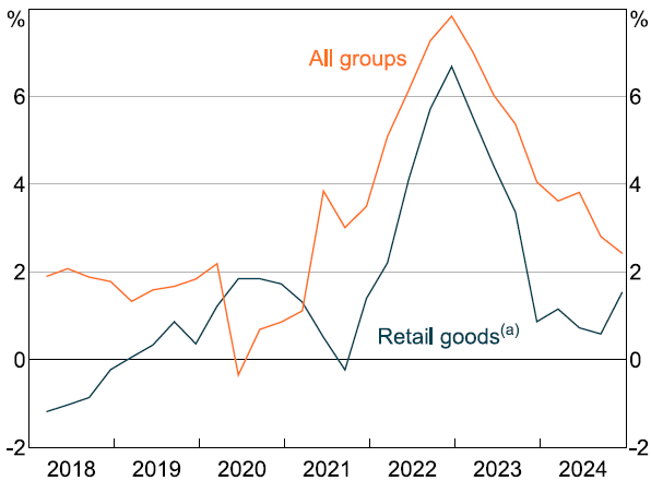
Note: (a) ABS CPI goods component excluding items not in web-scraped dataset: food & non-alcoholic beverages, tobacco, new dwellings, motor vehicles and automotive fuel.
Sources: ABS; Authors' calculations; RBA.
Monetary policymakers typically face a trade-off between lowering high inflation and supporting economic growth and employment, particularly in the wake of a supply shock, because reducing inflation in these circumstances requires curbing demand and activity to create slack and ease price pressures. In assessing the implications of our findings for monetary policy, we find that reduced price rigidity lessens the central bank's trade-off between stabilising inflation and real activity during large supply shocks. In this environment, policymakers can lower inflation with fewer real economic costs, suggesting a stronger focus on inflation stabilisation is warranted compared to a situation in which rigidity did not change.
We quantify these effects in the post-COVID-19 high-inflation period, using a so-called ‘optimal control’ exercise. This exercise uses the RBA's DSGE model to calculate the policy path that would have minimised deviations of inflation and unemployment from target, given the shocks that hit the economy, the structure of the model, and some set of simple fixed preferences for trading off between inflation and unemployment in the face of a supply shock. We compare these policy paths with and without the change in rigidity.
Relative to a scenario where rigidity remained unchanged, this exercise calls for policy that raises interest rates more aggressively – by up to around 40 basis points more than otherwise – followed by a sharper subsequent easing. Importantly, this does not imply that actual rates should have been higher than they were at the time. Our work compares these ‘optimal’ policy paths under different assumptions about price rigidity, rather than against the realised cash rate path. Moreover, the exercise uses a specific set of policy preferences around the trade-off between inflation and unemployment, which may differ from those used by policymakers during the high-inflation episode in 2022 and 2023. And the exercise relies on the structure of the model, which by its nature is a simplification of reality. Rather than prescribing a specific policy stance, our findings suggest that the observed decline in price rigidity would have made a front-loaded tightening more appealing for a central bank having to trade-off between inflation and unemployment, relative to the case where rigidity had not changed.
Beyond shedding light on this high-inflation episode, our paper contributes to the broader economic literature in several ways. First, it adds to the growing international empirical evidence on variability in price-setting frequency and nonlinear inflation dynamics. Our dataset covers a broader range of products than much of the existing literature using web-scraped data, including many discretionary and non-perishable items that may be less flexibly priced in normal times. Second, we are the first in this literature to apply formal duration modelling approaches to estimate price-setting frequency. These offer advantages over simpler ‘share of prices changing’ methods. Finally, we contribute to the relatively sparse literature on price-setting dynamics in Australia, focusing on a more recent period than previous studies and using web-scraped Australian data for the first time.
The objective of our analysis is to assess whether Australian firms' price-setting behaviour shifted over time within our dataset, and if so to explore the policy implications of those shifts. The remainder of the paper proceeds as follows. Section 2 reviews the existing literature in this area. Section 3 introduces our dataset. Section 4 introduces our preferred rigidity measure, price duration, and presents a time-varying measure estimated using a regression-based survival analysis approach that maps to the well-known Calvo parameter. Sections 5 and 6 explore the implications of changing price rigidity for inflation dynamics and monetary policy. Section 7 concludes with a discussion.
2. Literature Review
Modern macroeconomic models of the business cycle typically incorporate price rigidity to explain how fluctuations in nominal economic variables affect the real economy over time. A widely used framework is the Calvo pricing model, which is popular due to its tractability. This framework assumes that only a fixed proportion of firms can adjust their prices in each period (Calvo 1983). This frequency of price changes – often referred to as the ‘Calvo parameter’ – is usually treated as constant. This results in ‘time-dependent’ pricing, where firms decide to adjust prices on the basis of time rather than economic conditions. Consequently, nominal rigidity is also constant over time, implying a linear relationship between the size of a shock and its inflationary impact. [1]
This paper contributes to a substantial empirical literature that has emerged to assess price-setting dynamics. Early studies using CPI and scanner data found that prices were more flexible than assumed in standard macroeconomic models (e.g. Nakamura and Steinsson 2008; Klenow and Malin 2010). More recent work has leveraged web-scraped data, which provides advantages such as higher frequency, broader item coverage, and fewer measurement distortions than official statistics. Pioneering studies by Cavallo and Rigobon (2016) and Cavallo (2018) explore these benefits and show that web-scraped data can yield more accurate estimates of price-setting behaviour.
A general finding across this literature is that the frequency of price changes varies with economic conditions, challenging the fixed rigidity assumption in the Calvo framework. This evidence has motivated the development of models with state-dependent pricing, which better match observed behaviour. These models often imply nonlinear dynamics, where large shocks prompt more frequent price adjustments and therefore have larger and quicker effects on inflation.
Many of these models generate state-dependence by assuming that firms face fixed ‘menu’ costs when changing prices, so they adjust only when the benefit of doing so exceeds the cost (e.g. Alvarez, Le Bihan and Lippi 2016). Other approaches introduce costs of reviewing prices (e.g. Blanco et al 2024c) or costs of acquiring the information needed to choose optimal prices (e.g. Turen 2023). In all of these settings, shocks that push a firm's optimal price further from its current price strengthen the incentive to re-optimise. Firms therefore update their prices more frequently when economic conditions warrant it, giving rise to the state-dependent price setting observed in the data.
Recent papers have explored the importance of pricing dynamics in state-dependent models, particularly in the context of the pandemic (Dedola et al 2023; Auclert et al 2024; Cavallo, Lippi and Miyahara 2024; Blanco et al 2024a, 2024b, 2024c; Gautier et al 2026). These studies find that price rigidity tends to decline during large shocks, resulting in stronger inflation responses than predicted by time-dependent models. For example, Auclert et al (2024) show that while time- and state-dependent models yield similar inflation dynamics for small shocks in the euro area, state-dependent models produce markedly stronger responses when shocks are large.
The incorporation of state-dependent pricing into models also has important implications for monetary policy trade-offs. Karadi et al (2024), for instance, show that the trade-off between lowering inflation and preserving real economic activity in the United States is reduced during large shocks, as falling price rigidity steepens the Phillips curve. This implies that central banks should respond more aggressively to inflationary supply shocks than they would if price rigidity did not decrease.
Our paper contributes to the growing literature using prices microdata to examine price-setting shifts during and immediately after the COVID-19 period. These include Rudolf and Seiler (2022) for Switzerland; Montag and Villar (2025) for the United States, Henkel et al (2023) for euro area countries; Klein, Strömberg and Tysklind (2024) for Sweden; and Bilyk, Khan and Kostyshyna (2024) for Canada. Across these studies, the early pandemic (before inflation started rising significantly) generally saw relatively limited changes in the frequency of price adjustments. Studies covering the subsequent high-inflation period consistently document a strong increase in the frequency of price changes, driven mainly by more frequent price increases. This pattern suggests a shift toward more flexible pricing in response to large shocks, consistent with state-dependent pricing behaviour.[2]
Finally, our work builds on the limited literature examining price-setting dynamics in Australia. Using RBA firm survey data from 2000 to 2006, Cagliarini, Robinson and Tran (2010) find that prices are less rigid than typically assumed in structural macroeconomic models. Sutton (2017) uses CPI microdata from 2001 to 2017 and identifies moderate variation in price stickiness over time, with only modest increases in flexibility around the global financial crisis. Our paper extends these analyses, using a different data source – web-scraped prices – and focusing on a more recent period of heightened economic volatility with an emphasis on policy implications.
3. Data
3.1 Data structure and treatment
The most commonly used types of price microdata in empirical research include survey data underlying consumer and producer price indices, scanner data sourced from point-of-sale transactions and prices collected from firms' websites (‘web-scraped’ prices). A discussion of the strengths and limitations of these types of prices in a research context can be found in Cavallo (2018). The present paper uses a web-scraped dataset from the Australian Bureau of Statistics (ABS) Business Longitudinal Analysis Data Environment (BLADE), which captures advertised prices for every item offered on up to 61 large Australian retailers' websites. Prices were collected every few days between 2016 and 2023, with the number of firms sampled increasing over time. The dataset becomes sufficiently large to be reliable from 2018 and in total has around 549 million price observations for 13 million unique items. While data collection occurred frequently across the dataset, the timing of collections was irregular.
The dataset covers a broad range of retail items, such as apparel, homewares, and electronic goods, which together represent around 25 per cent of the Australian consumer price index (CPI) basket.[3] Retailers and items are de-identified, though their industry classification is known. Two key attributes of sampled firms are that: (i) they derive substantial revenue from both online and brick-and-mortar stores; and (ii) they account for a large share of total turnover in their respective industry subdivisions – around 30 per cent across sampled firms in each quarter on average. These characteristics support two assumptions underpinning our analysis: that online advertised prices generally reflect in-store prices; and that price-setting behaviour observed in the sample can be generalised to the broader retail sector.[4]
Compared to some recent studies of price-setting behaviour – such as Auclert et al (2024) and Cavallo et al (2024) – our dataset includes a broader range of products, particularly discretionary and durable goods. These types of goods should exhibit slower-evolving pricing and longer item life cycles. In this sense, our data is more comparable to that used in Dedola et al (2023) and Blanco et al (2024a, 2024b, 2024c), which cover a wider set of products and services. This allows us to explore how retail firms with pricing that is typically less flexible respond to large economic shocks, and what implications this has for inflation.
The collection method used by the ABS for our dataset ensures that the full pricing life cycle of each item is captured – from the first day an item is offered for purchase to the day it is removed. This typically results in a downward-sloping price path for items over time. Measuring prices over the full life cycle of a product differs from conventional CPI price collection methods, where items are periodically substituted to control for quality changes within product categories. As a result, our dataset is likely to contain a higher share of price decreases than CPI data, making it unsuitable for calculating CPI-like average inflation rate measures but well-suited for measuring the breadth of offered prices across the products firms sell and for gauging shifts in price-setting behaviour.
There is ongoing debate about whether changes in advertised (sales-inclusive) or ‘regular’ (non-sale) prices are more relevant for characterising price rigidity. While some researchers argue that only regular price changes reflect firms' responses to macroeconomic shocks or cost pressures, others contend that both regular and sales price changes may shift in response to economic fundamentals and that what ultimately matters for inflation dynamics are the prices at which consumers transact.[5] This latter view aligns with the construction of the Australian CPI, which incorporates all advertised prices, including sales prices.
Rather than taking a firm position, we present rigidity results for both advertised and regular prices. While the ABS dataset contains both, regular prices are only available from 2020 onward. To avoid relying on a short sample and ensure consistent classification of sales prices across firms and over time, we develop an algorithm to identify active sales based on pricing patterns.[6] Specifically, we identify ‘V-shaped’ sales, where a price drops and returns to an equal or higher level within three months, and ‘clearance’ sales, where a price falls by at least 25 per cent and exits the dataset within a month. We use these imputed regular and sales price series in our analysis rather than the reported regular price data, though we find that the reported and imputed regular price data generally align well over time (Figures A3 and A4).
Importantly, while the levels of measured price rigidity in our dataset may differ substantially depending on whether sales prices are included, the changes in rigidity over time are similar across both price types. Given this, concerns about the inclusion of sales prices do not materially affect our conclusions about how shifts in price rigidity influence inflation dynamics and policy decision-making.
A further description of our data, cleaning methodology and sales algorithm is provided in Appendix A.
3.2 Summary statistics
To validate the data, we first provide some basic statistics and visualisations. Figure 2 shows the distribution of the log size of price changes in the data over the full sample period. Advertised prices exhibit symmetrical peaks around large changes such as ±25, ±30, and ±40 per cent, alongside a central concentration of smaller changes between –5 and +10 per cent (Figure 2, top panel). Disaggregating into regular and sales prices reveals that most regular price changes fall between –5 and +10 per cent (middle panel), while sales-related price changes are typically larger, clustering around common discount rates such as ‘25 per cent off’ (bottom panel).[7] The symmetry in sales price changes reflects items being discounted temporarily and subsequently returning to full price. As noted above, there is a relatively large tail of negative price changes, compared to what we might see if using CPI microdata. This reflects that the web-scraped prices capture the full life cycle from when items are first offered for purchase to when they are retired.
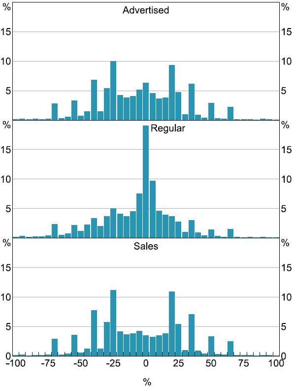
Notes: Item-weighted. x-axes are segmented in 5 percentage point intervals, where, for example, the zero bucket is changes between 0 and 5 per cent. Regular and sales prices are imputed using an algorithm that identifies sales patterns (see Appendix A).
Sources: ABS; Authors' calculations.
As a further validation, we look for evidence that the high-inflation period for goods is captured in our data. Given the nature of the data, rather than trying to recreate a CPI growth rate or focus on the size of price changes, we follow a number of other papers and look at the share of prices increasing and decreasing over each month (e.g. Bilyk et al 2024; Klein et al 2024). Specifically, we take the final price observation for each item in our data in each month and calculate the difference in the price compared to the end of the previous month. We then take the separate share of price increases and decreases out of all prices in each month, applying a 12-month trailing average to the resulting series to account for the highly seasonal nature of price setting. Subtracting decreases from increases provides a ‘relative frequency’ measure that can be used as a gauge for inflationary pressure. This approach abstracts from issues around life cycle pricing, as well as intra-month variation that is less relevant for observing the trend inflationary impulse.
We find that the share of price increases rose notably over 2022 and 2023, while the share of price decreases declined (Figure 3).[8] This means that the relative frequency of price increases rose substantially, in line with the increase in retail goods price inflation (Figure 4). More generally, this metric has a close association with retail goods price inflation, picking up slightly in 2020, before declining in 2021 alongside inflation. These results suggest that the dataset does effectively capture the inflationary impulse seen in the official Australian CPI in 2022 and 2023.
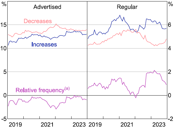
Notes:
12-month trailing averages. All series are averaged across firms using CPI weights.
(a) Relative frequency is calculated as the percentage point share of all end-of-month item prices that constitute an increase compared to the previous month less the share that constitute a decrease.
Sources: ABS; Authors' calculations.
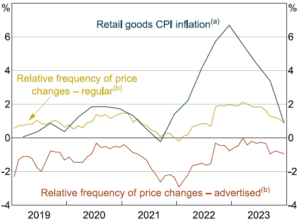
Notes:
(a) Year-ended growth in the ABS CPI goods component excluding items not in web-scraped dataset: food & non-alcoholic beverages, tobacco, new dwellings, motor vehicles and automotive fuel.
(b) Relative frequency is calculated as the percentage point share of all end-of-month prices that constitute an increase compared to the previous month less the share that constitute a decrease. Shares of increases and decreases are calculated as 12-month trailing averages. Averaged across firms in the web-scraped dataset using CPI weights.
Sources: ABS; Authors' calculations.
4. Measuring Price Rigidity
Several ways of measuring price rigidity have been proposed in the literature. One is by simply looking at the share of prices that change in a month. However, this does not account for cases where prices may change multiple times in a month, which would abstract away from the richness of our high-frequency price data.[9] Moreover, such measures do not account for how long a price has remained unchanged before adjusting – an important dimension of rigidity. Another approach is to look at the kurtosis of the distribution of price changes, which has been shown to provide a sufficient statistic for parameterising macro models with state-dependent pricing mechanisms (Alvarez et al 2016). However, kurtosis measures can be heavily affected by sample changes and noise.
Instead, we focus on measures of price duration – how many days since the price last changed. These overcome some of the above limitations and are well suited to our dataset. Moreover, they have a direct mapping to objects of interest in standard macroeconomic models of the business cycle, such as Calvo parameters.
4.1 Simple price duration measures
We start by showing the average number of days since an item last recorded a price change for all items that had a change in price. Following a period of relative stability through mid-2021, advertised and regular price durations rose as goods inflation rose, with longer intervals between changes on average (Figure 5, top panel). These results seem counterintuitive. However, they are largely explained by compositional effects. As inflation picked up, many prices in our dataset that had remained unchanged for extended periods – sometimes several years – began to adjust. The entry of these long-lived prices into the sample of changing prices increased the mean duration, even though firms were likely changing prices more frequently overall.
To see this, we can look at the distribution of price durations. The rise in average duration was concentrated in the upper tail of the distribution (e.g. the 75th percentile and above), while the median remained relatively stable (Figure 5, middle and bottom panels). The fact that long-stable prices began adjusting more often provides some initial evidence that price-setting frequency increased during the high-inflation period.
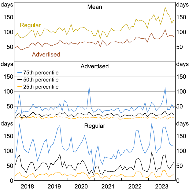
Note: Item-weighted.
Sources: ABS; Authors' calculations.
4.2 Survival analysis methodology
To explore this more formally we perform a survival analysis to estimate the probability that a price remains unchanged over time. This approach has several advantages. First, survival analysis incorporates the full set of price spells in the data, including prices that do not change.[10] This makes it less sensitive to compositional changes in the sample driven by changes in very long-lived prices. Second, the regression-based framework allows us to formally test whether changes in rigidity over time are statistically significant. Third, survival models can control for firm-level heterogeneity and item censoring (where items enter or exit the sample mid-spell).
We use a parametric survival model with an exponential survival function, which assumes a constant hazard rate, that is, the probability of a price persisting is independent of information about how long it has been since that price last changed.[11] This assumption aligns with the Calvo pricing model commonly used in DSGE frameworks, allowing us (through a simple conversion) to interpret the estimated survival rates of prices as Calvo probabilities.
The model is estimated by maximum likelihood over the full set of price spells, accounting for two key features of the data:[12]
- Firm fixed effects: these control for persistent differences in pricing behaviour across retailers, helping isolate within-firm changes over time and abstract from changes in the composition of firms in the sample.
- Censoring: to address left censoring (e.g. unknown price history before an item enters the sample), we exclude the first observed spell for each item. The model also handles right censoring, where items exit the sample without a price change by incorporating this possibility into the likelihood function.
In our baseline specification, price survival probabilities are allowed to vary by the quarter or year in which a price spell begins.[13] The estimation takes the following form:
where:
- Sir (t|xj) is the survival function giving a probability that the price of item i offered by retailer r remains unchanged for at least t days conditional on the year or quarter in which the price is observed xj,
- is a retailer-specific baseline hazard (rigidity) rate capturing firm fixed effects,
- xj is a vector of indicator variables for the year or quarter associated with the end of a given price spell, and
- is a vector of coefficients on these time indicators, capturing period-specific survival rates across firms.
The survival function gives the probability that a price does not change up to a given point in time for each year or quarter in which underlying prices were observed. To make these results comparable to the Calvo parameter commonly used in macroeconomic models – which is expressed as the probability of a price remaining unchanged over one quarter – they are scaled to reflect the probability of prices remaining unchanged after 90 days (i.e. we set t = 90).[14]
4.3 Survival analysis results
We estimate price rigidity separately for advertised and regular prices. As expected, regular prices are more rigid, reflecting the high prevalence of temporary discounting in advertised prices. On average, the probability that a regular price remains unchanged after one quarter is 51 per cent, compared with 14 per cent for advertised prices (Figure 6).[15] These estimates are broadly consistent with empirical evidence from Sutton (2017). However, they imply greater price flexibility than standard macroeconomic models – an observation common in the international literature.[16] For example, the RBA's DSGE model implies around 70 per cent of prices remain unchanged each quarter in the non-resource tradeables sector (which best aligns with our sample), and around 85 per cent on average across the broader economy.
We also find meaningful variation in rigidity over time. Regular prices became more rigid and less likely to change during the early pandemic period, with the probability of remaining unchanged rising by around 10 percentage points between 2019 and 2021. This was less evident for advertised prices, suggesting that firms were, in relative terms, relying more on discounting as a method for adjusting prices. This is consistent with heightened uncertainty evident during this period, which may have made firms relatively less willing to make more permanent price changes.[17]
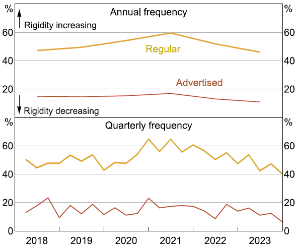
Notes: Item-weighted. Shading shows 95 per cent confidence intervals.
Sources: ABS; Authors' calculations.
From 2022 onward, as general retail goods inflation accelerated, both regular and advertised prices became significantly more flexible: by the end of the sample the share of advertised and regular prices remaining unchanged over a quarter was 25 and 7 per cent lower, respectively, than before the pandemic. This suggests that when faced with large inflationary shocks and rising input costs from 2022, firms started changing prices more regularly, including by making more permanent changes.[18] This is consistent with international evidence that price rigidity tends to decline during high-inflation periods (see Cavallo et al (2024) and Gagliardone et al (2025)). It is also broadly in line with comparable overseas estimates, such as those documented using European CPI microdata in Gautier et al (2026).
5. How Shifts in Price Rigidity Affect Inflation Dynamics
Having established in Section 4 that firms' price rigidity changed materially over the pandemic period and immediately after, we now assess whether these changes had meaningful implications for inflation dynamics. Specifically, we ask: if price rigidity declined between 2019 – our proxy for ‘normal times’ – and 2023 in line with our empirical evidence, how would this change have altered the transmission of shocks to inflation?
There are several ways to explore this question. One approach would be to build a new macroeconomic model calibrated to our microdata estimates. Another would be to incorporate our results into the RBA's existing benchmark DSGE model, which is used for policy analysis.[19] We adopt the latter approach, as it allows us to assess the implications of changing price rigidity within a framework familiar to policymakers. This helps bridge the gap between micro-level evidence and benchmark policy tools. Our exercise is similar in spirit to Gelain and Lopez (2024), who adapt the Federal Reserve's linear model frameworks to better capture inflation dynamics around the pandemic.
We focus on variation in the Calvo parameter – the probability that a firm does not adjust its price in a given period – which we estimated in Section 4 using survival analysis. Because the level of our estimated Calvo parameters differs from that used in the baseline DSGE model, we adjust the slope of the Phillips curve using the change in rigidity between 2019 and the peak of the inflation surge in 2023.[20] This embeds an assumption that ‘normal’ price rigidity in our data is best represented by the observed rigidity probability immediately prior to the start of the COVID-19 pandemic, and that the change in rigidity was similar across all goods and services in the CPI. We think this is broadly reasonable given the extended period of price stability prior to 2020. An alternative approach would be to test the effect of the shift in rigidity from its highest point in 2021 (immediately prior to the inflation surge) to its lowest point in the data during the surge in 2023. However, this would be less in line with the intent of comparing price rigidity at the peak of an inflationary episode to the normal rigidity embedded in our benchmark policy model.
5.1 Adjusting the slope of the Phillips curve
The RBA's DSGE model uses a Rotemberg-type price adjustment mechanism. To incorporate our Calvo-based rigidity estimates, we exploit the well-known equivalence between Rotemberg and Calvo pricing under a first-order approximation around the zero-inflation steady state.[21] This allows us to adjust the Phillips curve slope in the model using our estimated Calvo parameters. Specifically, the Phillips curve in the model can be expressed as:
where:
- is inflation,
- MCt is marginal costs,
- is a cost-push shock,
- is the slope of the Phillips curve, which is defined as:
Here, is the discount factor, is the degree of price indexation and is the Calvo parameter (the share of prices that remain unchanged in each period). Given the direct estimates of in the RBA's model and the parameters and , we can back out . We can then adjust using our microdata estimates to create an alternate Phillips curve slope .[22]
One natural question is how to map our estimated Calvo parameters into the model, given that there are levels differences between the estimated slopes in our empirical data and those embedded in the various sectors of the DSGE model. We test two approaches: one based on the absolute change in our estimate of rigidity (percentage points), and another based on the proportional change (per cent). These serve as lower and upper bounds for our analysis (Table 1).
| Advertised prices | Regular prices | |
|---|---|---|
| 2019 | 14.6 | 49.5 |
| 2023 | 10.9 | 46.1 |
| Lower bound difference (ppt) | −3.7 | −3.4 |
| Upper bound difference (%) | −25.3 | −6.9 |
| Sources: ABS; Authors' calculations. | ||
Rather than having a single Phillips curve, the DSGE model includes separate Phillips curves for each of five sectors: resources, tradeables, non-tradeables, imports and housing. We uniformly apply the observed variations in price rigidity between 2019 and 2023 to the slope of each curve; that is, we treat the observed shift in retail price rigidity as representative of a shift in economy-wide rigidity. Although this may seem a somewhat strong assumption, it is not obvious a priori whether other sectors would have experienced larger or smaller shifts. For example, applying the adjustment only to the tradeables sector would imply no changes in rigidity elsewhere in the economy, which is at least as strong an assumption as distributing the observed shift evenly across sectors.[23] While this choice affects the precise magnitudes of our quantitative results, it does not alter their qualitative implications.
5.2 Illustrating the role of price rigidity in the DSGE framework
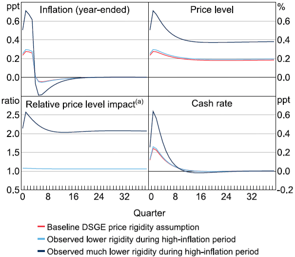
To illustrate the impact of price rigidity on inflation dynamics, we simulate a 1 per cent increase in the cost of foreign imports (i.e. a cost-push shock) in the DSGE model, using our estimated range of Calvo parameters for regular prices. We find that lower price rigidity leads to a stronger and faster inflation response. Specifically, the initial pass-through of the shock to year-ended inflation is higher by between 0.03 and 0.28 percentage points (Figure 7). The long-run impact on the price level also increases, rising from around 0.2 per cent under baseline rigidity to as much as 0.32 per cent under lower rigidity – an increase of nearly 75 per cent.[24]
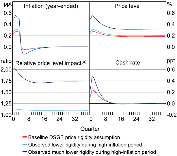
Notes:
100 basis point positive shock in the price of foreign imports.
(a) Ratio of the price level impact from the shock using alternative rigidity assumption over impact using baseline rigidity.
Sources: ABS; Authors' calculations.
Given the DSGE model's Taylor rule, which includes inflation and a measure of real activity, this larger inflation response translates into a more aggressive policy interest rate path. The cash rate rises by between 3 and 25 basis points more in the first year compared to the baseline. Results are similar – but the cash rate increase is somewhat larger – when using the range of Calvo parameters estimated for advertised prices, which include temporary discounts and tend to be more flexible (Figure D1).
5.3 Forecasting inflation with time-varying price rigidity
The previous subsection illustrated how changes in price rigidity affect the transmission of a single shock. To assess the practical relevance of these changes, we now ask: if price rigidity declined between 2019 and 2023 as our estimates suggest, how much would this have affected model-based inflation forecasts during the post-pandemic surge?
To answer this, we conduct a scenario forecasting exercise using the DSGE model. We treat our microdata-based estimates of shifts in price rigidity as true and adjust the slope of the Phillips curve accordingly. We then use the model to recover the set of shocks that must have hit the economy to generate observed outcomes. Finally, we simulate the model forward from the start of 2022 using these estimated shocks but revert the Phillips curve slope to its baseline value. Comparing the resulting inflation forecasts to actual outcomes allows us to isolate the impact of misspecified price rigidity in the simulation. This approach is similar to that of De Fiore et al (2023), who use it to evaluate alternative monetary policy frameworks during the post-pandemic inflation period.[25] The exercise can be thought of as asking: how wrong would forecasters who only use the DSGE model have been if they had known all the shocks that were going to hit the economy, but didn't account for the fact that price rigidity had changed?
The DSGE model can be represented in its vector autoregression (VAR) form:
where:
- Yt is the vector of endogenous variables,
- is a matrix linking past values to current outcomes based on the model parameters,
- are structural economic shocks,
- is a matrix capturing the transmission of shocks based on the model parameters.
Changing the Phillips curve slope (via ) alters both and . Using our lower rigidity estimates, we denote the adjusted matrices as and , and the recovered shocks as . The model then becomes:
We take this set of equations to be the true structure of the economy, and so are the true structural shocks that were hitting the economy during the period, given the observed data.
With these true shocks in hand, we can then revert to the original model structure from 2022 onwards and calculate what forecasters might have expected inflation to be if they knew the shocks hitting the economy but had the wrong model structure and rigidity. The counterfactual conditions would be:
The difference between observed and counterfactual outcomes, , gives an estimate of the forecast error attributable to misspecified price rigidity.[26]
5.3.1 Results
Figure 8 shows actual year-ended headline inflation alongside model-predicted inflation using the upper and lower bounds of our estimated rigidity decline. Even assuming perfect knowledge of the shocks, failing to account for the decline in price rigidity would have led the DSGE model to under-predict inflation by between 0.42 and 1.24 percentage points one year ahead. The peak of inflation would also appear slightly more persistent and delayed. The magnitude of these effects are broadly in line with findings in Gautier et al (2026), who argue that failing to account for changes in price-setting frequency in Europe during the post-pandemic high-inflation period would have led to inflation predictions being 1 percentage point lower.
These findings suggest that ignoring time variation in price rigidity – particularly during periods of large cost shocks – can lead to significant forecast errors. While our analysis is based on a DSGE framework, the implications are broader. Many forecasting models, including single-equation Phillips curves commonly used in public and private sector institutions, assume a fixed Phillips curve slope. Our results highlight the importance of allowing for time-varying price-setting frequencies when inflation dynamics are shifting rapidly and demonstrate that this was critically important during the recent inflationary episode.
As a supplementary exercise, we also tested whether varying the assumed degree of price rigidity affects the model's decomposition of inflation into supply and demand shocks. The results suggest minimal sensitivity to this assumption. See Appendix E for details.
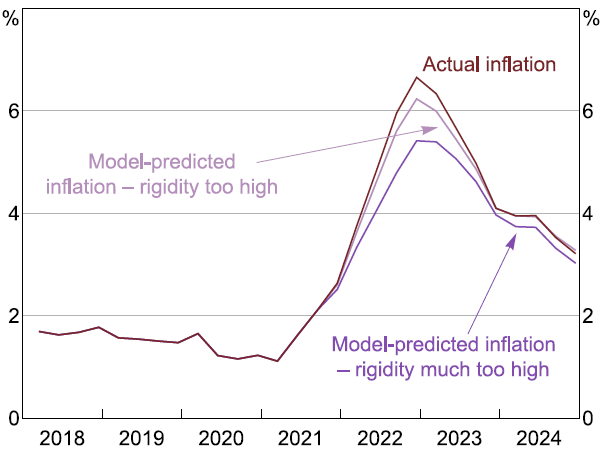
Note: Actual inflation rate versus predicted path of inflation if price rigidity in the model was overestimated.
Sources: ABS; Authors' calculations.
6. How Shifts in Price Rigidity Affect Monetary Policy
Changes in price-setting behaviour can have important implications for monetary policy. If price rigidity varies over time, then the transmission of monetary policy – and the trade-offs faced by policymakers, particularly during supply-side shocks – may also change.
In this section, we explore the implications of changes in price rigidity for monetary policy transmission, trade-offs and strategy. We conduct two exercises. First, we undertake a so-called optimal control exercise, calculating the policy paths that would have minimised (weighted) deviations of inflation and unemployment from target during the 2022–2023 high-inflation period under baseline model rigidity and under the lower rigidity observed in that period. Second, we examine how the optimal weights (those that minimise weighted deviations of inflation and unemployment) in a simple Taylor rule change as rigidity declines. This latter exercise is especially relevant in the context of supply-side shocks, where inflation and output move in opposite directions, creating a sharper policy trade-off. In contrast, demand-driven shocks typically move inflation and output in the same direction, making the implications of changing rigidity for those trade-offs less pronounced.
6.1 Transmission of monetary shocks under varying rigidity assumptions
To motivate the analysis, we first simulate the impact of a 100 basis point monetary policy tightening shock under baseline and lower rigidity assumptions. The results show that when prices are more flexible, the disinflationary effect of a given rate increase is stronger (Figure 9). Crucially, this stronger inflation response is achieved without a larger decline in output. A steeper Phillips curve means that a given reduction in real activity translates into a larger fall in inflation. As a result, the trade-off between stabilising inflation and supporting real output is reduced.
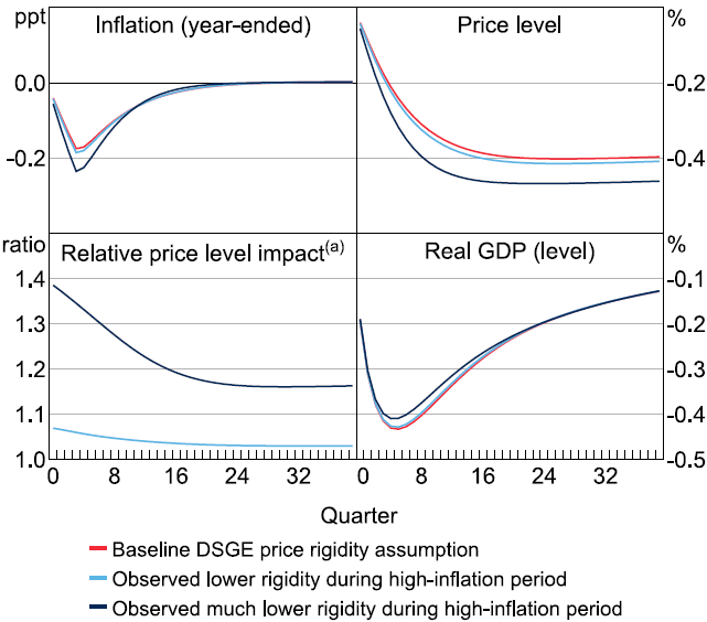
Notes:
100 basis point positive shock in the cash rate.
(a) Ratio of the price level impact from the shock using alternative rigidity assumptions over impact using baseline rigidity.
Sources: ABS; Authors' calculations.
6.2 Optimal control exercises under varying price rigidity assumptions
We now examine how shifts in price rigidity affect monetary policy trade-offs and strategy. To do this, we implement an optimal control exercise using the DSGE model. Unlike a fixed policy rule approach (e.g. estimating a Taylor rule), optimal control calculates the path for the cash rate that minimises a standard policy loss function, given the shocks that hit the economy. This is a common method used by policymakers (e.g. Lowe and Ellis 1997; Adolfson et al 2011).
6.2.1 Methodology
For our analysis we assume that the loss function places equal weight on stabilising inflation, output (as a proxy for unemployment) and interest rate smoothing. Formally:
where:
- aj are the policy-relevant variables (inflation, output gap, and change in the nominal interest rate),
- are their respective ‘targets’ (2.5 per cent for inflation, 0 percentage points for both output gap and interest rate changes),[27]
- are the weights assigned to each variable,
- is the discount factor (set to 0.9996),
- the summation covers the period from March 2022 to December 2024.
Inflation and interest rate changes are each assigned a weight of 1. The output gap is weighted at 1/64, which equates a 1 percentage point deviation in inflation to a 1 percentage point unemployment gap, based on Okun's law. This implies equal weighting across inflation, unemployment, and interest rate volatility in the loss function.
We focus on unanticipated monetary policy shocks and do not compare the paths generated from this exercise with the actual policy response during the period, as this would not be a like-for-like comparison. Policymakers may have used a different loss function, and the model incorporates ex post information that was not available in real time. Instead, we compare paths under different rigidity assumptions to draw general lessons about how monetary policy should respond when price-setting behaviour changes, ceteris paribus.
6.2.2 Results
Figure 10 shows the policy paths from the exercise under baseline and lower rigidity assumptions. When prices are less rigid, the interest rate rises more aggressively in response to inflationary shocks. The cash rate peaks between 10 and 41 basis points higher than under baseline rigidity within the first year, resulting in substantially lower inflation.[28]
While output growth also declines slightly more than under the baseline, the trade-off is more favourable: the additional disinflation is achieved with only a modest additional fall in output. This reflects the steeper Phillips curve under lower rigidity, which allows inflation to be stabilised more effectively for a given change in real activity.
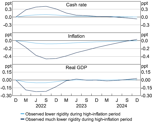
Notes: Cash rate path from optimal control exercise and associated inflation and real GDP outcomes under alternative assumptions about price rigidity. Results are shown relative to those obtained using the baseline price rigidity estimate embedded in the model. Inflation and real GDP growth are annualised growth rates.
Sources: ABS; Authors' calculations.
Overall, our findings suggest that when price-setting frequencies pick up – particularly during supply-side inflationary shocks – monetary policy can be tightened more aggressively to achieve faster disinflation with limited additional cost to output and unemployment. These results are consistent with those described in Karadi et al (2024), who conduct a similar exercise for the 2022-2023 US inflation surge using a model with state-dependent menu cost rigidities.
6.3 Optimal simple rules under different rigidity assumptions
While optimal control exercises provide a full policy path under a particular scenario, central banks often rely on simple policy rules – such as the Taylor rule – for communication, forecasting, and operational guidance. The Taylor rule prescribes a policy interest rate response given deviations in inflation and output from their targets (Taylor 1993). If price rigidity changes over time, and so the trade-off between inflation and unemployment changes, this could alter how aggressively policymakers want to respond to inflation and output fluctuations, and therefore the preferred weights in the rule.
To explore this, we assess how the coefficients in a standard Taylor rule that minimise a loss function vary under different assumptions about price rigidity. This helps quantify how monetary policy trade-offs evolve when firms adjust prices more flexibly, particularly during supply-side shocks.
6.3.1 Methodology
The Taylor rule specification embedded in the RBA's DSGE model takes the following form:
where:
- it is the nominal interest rate,
- it–1 is the lagged interest rate,
- r* is the neutral real interest rate,
- is the two-quarter-average inflation rate,
- is the inflation target,
- is the two-quarter-average GDP growth rate,
- and are the policy response coefficients to inflation and output, respectively,
- is the interest rate smoothing parameter,
- is a monetary policy shock.
To estimate how the values of and that minimise losses vary with price rigidity, we simulate the DSGE model under different Calvo parameters (as estimated in Section 4). For each rigidity setting, we solve for the Taylor rule coefficients that minimise the same policy loss function used in Section 6.2, subject to the model's structure and shock variances. In this sense, this exercise is thinking about what general rule would be optimal on average over all time under the different rigidities.[29]
6.3.2 Results
Under the baseline rigidity setting in the model, the loss-minimising weight on inflation is approximately 1.8 times the weight on output. When rigidity is lowered in line with observed changes during the post-pandemic inflation, this ratio increases to between 1.9 and 2.4 – a rise of 5 to 33 per cent.[30] These results are consistent with our earlier findings. When prices are more flexible, inflation responds more to changes in activity and the Phillips curve becomes steeper. As a result, placing greater emphasis on inflation in the policy rule is preferred. Our estimated ratios provide a simple metric for thinking about how the central bank's policy considerations might shift during large economic shocks that cause periods of elevated inflation and lower price rigidity.
7. Conclusion
Our analysis shows that the large supply shocks of the late pandemic period coincided with a decline in price rigidity, as firms became more willing to adjust prices. This shift contributed meaningfully to the sharp rise in inflation in 2022 and 2023.
The observed tendency for price rigidity to decline during large shocks has important implications for macroeconomic modelling and policy. First, inflation may accelerate more rapidly than predicted by standard linear models, requiring forecasters – including central banks – to account for more flexible price-setting behaviour. Second, as rigidity falls, the Phillips curve steepens, reducing the trade-off between inflation and output. This means that, all else equal, central banks facing large supply-side inflationary shocks can raise interest rates more aggressively and achieve inflation objectives more quickly, with limited additional costs to economic activity.
Applying these insights in real time is challenging. Prices microdata are not currently available on a timely basis in many countries, including Australia, and the nature of shocks during turbulent periods can be difficult to identify. Policymakers must therefore rely on informed judgement to assess whether firms are adjusting prices more frequently. Business liaison and business surveys may offer valuable real-time signals in these periods.
Accurate identification of the type of shock hitting the economy is also critical. The policy implications we describe for periods of lower price rigidity are most relevant for supply-side shocks, where inflation and output move in opposite directions. In contrast, demand shocks typically push both inflation and output in the same direction, making the policy trade-off less relevant. This underscores the importance of robust shock identification, as discussed in Beckers, Hambur and Williams (2023).
One way to improve forecasting accuracy under shifting price-setting behaviour is to expand the set of models used in policy analysis. Models with state-dependent pricing allow firms' responsiveness to vary with the size of economic shocks and can be calibrated using empirical moments from microdata – such as those estimated in this paper.
In the absence of timely data or formal models that explicitly capture changing rigidity, policymakers must lean more heavily on informed assessment. In these instances, the findings in this paper offer an intuitive evidence-based guide to how price-setting behaviour is likely to evolve during large supply shocks and how these changes affect inflation dynamics and the design of monetary policy responses.
Appendix A: Data, Cleaning and Sales Algorithm
A.1 Data description
A.1.1 Data collection
The raw data consists of prices for retail goods listed on the websites of major Australian retailers. These were collected by the Australian Bureau of Statistics (ABS) every few days between the start of 2016 and end of 2023. In general, the collection process involved taking the price of every item listed on a given retailer's website. The ABS performed some additional cleaning to reduce the likelihood that price collections were made for duplicates of the same item; however, in some instances it is possible that very similar items are recorded separately.[31]
Price collection dates vary by firm, and the frequency of price collections for a given firm may be irregular. For example, all prices for the items of a given firm might be collected on one date, then two days later, then four days later, then three days later, etc. The median frequency of price collections per item across firms is around six per month; this varies over time but generally increases over the sample (Figure A1).[32] Because of this, our main analysis of price rigidity uses a survival analysis method that accounts for bias from the irregular timing and frequency of price collections.
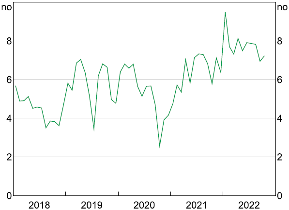
Sources: ABS; Authors' calculations.
A.1.2 Data fields
Data fields available for each retailer include a unique item number that is consistent across collection dates, the date of each price observation and up to three types of prices: ‘advertised’ prices, which are the current retail price of the item offered to consumers on that date (this may or may not be a discounted price); ‘regular’ prices, which are the undiscounted price of the item; and ‘sales’ prices, which are the price of the item if a sales event is active (Table A1). Advertised prices are available from the start of the dataset, while regular and sales prices are only available from 2020. The recording of regular and sales prices in the raw data reflects the classification of these price types by the retailers themselves as per their website. This means that there may be inconsistency in how sales activity is recorded across firms. For this reason, we standardise the definition of regular and sales prices across firms using the sales algorithm described in Section A.3.
| Retailer code | Retailer group | Item code | Date | Advertised price | Regular price | Sale price |
|---|---|---|---|---|---|---|
| 5 | clothing | 1 | 01/01/2020 | 20 | ||
| 5 | clothing | 1 | 03/01/2020 | 15 | ||
| 5 | clothing | 1 | 06/01/2020 | 15 | 20 | 15 |
| 5 | clothing | 2 | 01/01/2020 | 10 | ||
| 5 | clothing | 2 | 03/01/2020 | 12 | ||
| 5 | clothing | 2 | 06/01/2020 | 12 |
A.1.3 Firm and product types
The presence and total number of firms captured in the dataset varies over time, with the number of firms being too small to provide comfort about statistical validity of the sample prior to 2018. Between 2018 and 2023, the average number of firms present in each month is 53 and the total number of unique firms is 61 (Figure A2). Each firm in the dataset is deidentified, although a ‘retailer group’ variable corresponding to the broad retail category of each firm is provided. The set of retailer categories is: alcohol, automotive, clothing, cosmetics, department store, electrical, eyewear, footwear, furniture, hardware, homewares, jewellery, magazines, and pharmaceuticals.
Apart from the general category of the retailer and a deidentified product code, no information about the nature of a given sampled product is available in the dataset. This means that analysis at a more granular ‘product type’ level is not possible. That said, the ABS has collected information about the product type of items and may make this available in some form in the future.
ABS confidentiality requirements restrict the amount of information that can be shared about the pricing behaviour of individual firms present in the data.
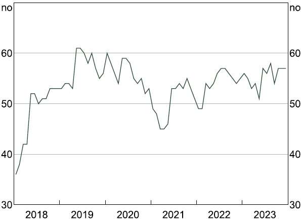
Sources: ABS; Authors' calculations.
A.1.4 CPI weighting
Where appropriate, measures constructed as a part of our analysis are weighted using weights derived from mapping retailer categories to their approximate category matches in the consumer price index. This mapping is shown in Table A2. Where several retailers are part of the same category, we split their category weight evenly amongst them.
| Retailer group | Nearest analogous ABS CPI expenditure groupings | CPI weight used in analysis(a) |
|---|---|---|
| Alcohol | Alcoholic beverages | 5.0 |
| Automotive | Spare parts and accessories for motor vehicles | 0.8 |
| Clothing | Garments | 2.0 |
| Cosmetics | Personal care products | 0.9 |
| Department store | Combination of: household textiles; household appliances, utensils & tools; clothing & footwear | 5.3 |
| Electrical | Combination of: major household appliances; small electric household appliances; audio, visual & computing equipment | 1.9 |
| Eyewear | Accessories | 0.7 |
| Footwear | Footwear | 0.5 |
| Furniture | Furniture | 1.4 |
| Hardware | Combination of: tools & equipment for house and garden; maintenance & repair of the dwelling | 2.5 |
| Homewares | Combination of: household appliances, utensils & tools; household textiles | 2.0 |
| Jewellery | Accessories | 0.7 |
| Magazines | Newspapers, magazines & stationery | 0.4 |
| Pharmaceuticals | Pharmaceutical products | 1.0 |
|
Note: (a) Based on average annual weights for mapped CPI expenditure groupings between 2018 and 2023. Sources: ABS; Authors' calculations. |
||
A.2 Data cleaning
Price changes are measured between two consecutive observations in the dataset and are calculated in log difference terms. For the survival analysis, we drop price observations that may be stale, which we define as when the distance between two price observations is 30 days or more. As noted in Section 4.2, we also drop the first price spell for each item to avoid the possibility of left censoring. Further cleaning of our imputed regular prices series is described in the next section. Apart from these measures, we include all price observations in the dataset.
A.3 Sales algorithm
Firm-reported regular and sales prices are available in our dataset from late 2020. To extend these series back to the start of 2018 and ensure a consistent definition of sales prices across firms, we develop an algorithm that identifies temporary and clearance sales based on observed price patterns.
Our approach follows the methodology introduced by Nakamura and Steinsson (2008) and further developed in Gautier et al (2024). The algorithm classifies price changes as either regular or discount-related by identifying specific patterns in the evolution of advertised prices over time:
- Temporary (or ‘V-shaped’) sales are flagged when the advertised price of an item falls and then returns to an equal or higher level within three months. To ensure any return to full price can be observed for all items, we exclude prices recorded within the last three months in which a firm appears in the dataset.
- A temporary sale flag is removed if a post-discounting price is followed by another price decline within 14 days. This helps to avoid misclassifying volatile pricing behaviour as discounting activity.
- Clearance sales are identified when an advertised price falls by at least 25 per cent and the item exits the dataset within one month. Prices within one month of the end of a firm's data are excluded from the data to ensure the exit condition can be verified.[33]
To assess the performance of the algorithm, we compare our imputed regular and sales prices series to ABS-recorded full and discount prices series available from late 2020 onwards (Figures A3 and A4). The imputed and ABS-recorded series generally align well in level and trend. However, at disaggregated levels, the ABS-recorded data suggest some inconsistencies in how firms distinguish between regular and sales prices, likely reflecting variation in how retailers label discounts on their websites or how the web scraper captured this information.
A key advantage of our algorithm is that it applies a uniform definition of sales events across all firms. By focusing on the underlying structure of price changes – rather than relying on retailer-provided labelling – the algorithm ensures that discounts are identified consistently, regardless of how they are attributed in the source data.
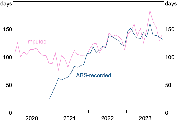
Notes: Item-weighted. Average number of days since prices last changed, conditional on a change having occurred.
Sources: ABS; Authors' calculations.
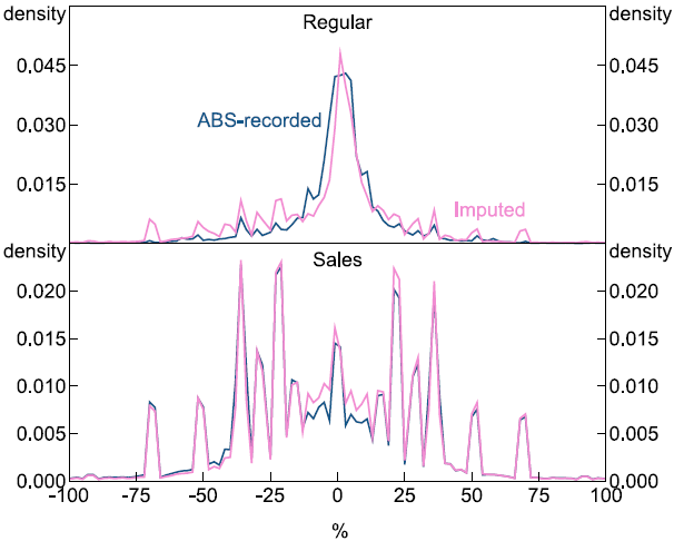
Notes: Item-weighted distribution of log price changes by size estimated by kernel density. The density is evaluated on the x-axes in 2 percentage point intervals. For example, the value plotted around zero corresponds to price changes in the interval –1 to 1 per cent.
Sources: ABS; Authors' calculations.
Appendix B: Additional Analysis of the Size of Price Changes
We document how the distribution of price changes shift over time. At the onset of the pandemic, the distribution of both advertised and regular price changes became more dispersed, with increased weight in the tails – indicating a higher incidence of large price increases and decreases (Figures B1 and B2).[34] This is reflected in a notable rise in the kurtosis of price changes around 2021 in both price measures (Table B1). The increase in kurtosis suggests a shift toward larger price adjustments, which coincided with a sharp drop in demand and heightened economic uncertainty.
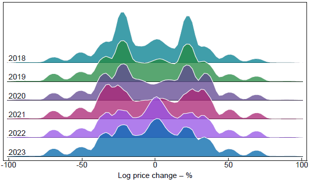
Sources: ABS; Authors' calculations.
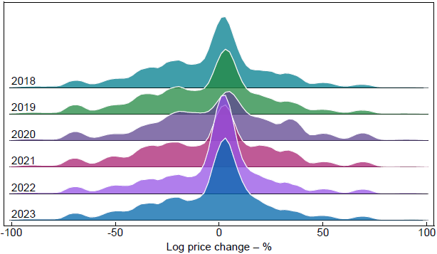
Note: Imputed regular prices.
Sources: ABS; Authors' calculations.
| Advertised | Regular | ||||
|---|---|---|---|---|---|
| Item-weighted | Firm-weighted(a) | Item-weighted | Firm-weighted(a) | ||
| 2018 | 10 | 12 | 11 | 21 | |
| 2019 | 8 | 10 | 10 | 20 | |
| 2020 | 7 | 11 | 9 | 17 | |
| 2021 | 15 | 18 | 48 | 22 | |
| 2022 | 6 | 14 | 11 | 27 | |
| 2023 | 7 | 12 | 12 | 18 | |
|
Note: (a) Cross-firm CPI-weighted mean calculated using fixed effects regressions to control for volatility in firm composition. Sources: ABS; Authors' calculations. |
|||||
During the high-inflation period, the distribution of regular price changes became more centralised, with a higher frequency of smaller adjustments and a decline in kurtosis. This pattern is consistent with theoretical and empirical work showing that higher inflation reduces the relative cost of frequent price changes, leading firms to adjust prices more often but potentially by smaller amounts.[35] However, interpreting these shifts is not straightforward. While visual inspection suggests a greater share of small price changes during the high-inflation period, kurtosis levels are broadly similar to pre-pandemic values. This makes it difficult to draw firm conclusions from these measures about whether price rigidity was ultimately higher or lower than before the pandemic. Moreover, changes in the nature of the shocks driving marginal costs could also influence the distribution of price changes.
This highlights some of the challenges in using distributional statistics to infer changes in price-setting behaviour. Estimates of kurtosis are highly sensitive to changes in sample composition and outlier values. For example, combining subgroups with different variances – even if each has the same kurtosis – can inflate the overall measure. While our firm-weighted metrics attempt to control for compositional shifts by focusing on within-firm changes, variation in the number of items per firm could also still affect results. More broadly, measurement error – whether from prices being captured inaccurately or irregular data collection – can bias kurtosis estimates. So while our distributional measures offer useful insights, they should be interpreted with caution and complemented by more robust methods as in our Section 4.
Appendix C: Survival Analysis Regression Results
The tables below include coefficients from the survival analysis that correspond to the beta term in Equation (1). Transformation of a given coefficient to a cross-sample quarter frequency Calvo parameter equivalent is achieved via:
| Advertised prices | Regular prices | |
|---|---|---|
| 2018 | −3.871*** [−3.866, −3.876] |
−4.800*** [−4.791, −4.809] |
| 2019 | −3.859*** [−3.855, −3.864] |
−4.866*** [−4.857, −4.875] |
| 2020 | −3.884*** [−3.879, −3.888] |
−5.005*** [−4.996, −5.014] |
| 2021 | −3.940*** [−3.935, −3.945] |
−5.171*** [−5.163, −5.180] |
| 2022 | −3.804*** [−3.800, −3.809] |
−4.936*** [−4.927, −4.945] |
| 2023 | −3.720*** [−3.715, −3.725] |
−4.769*** [−4.760, −4.778] |
| No of observations | 49,916,224 | 13,139,762 |
|
Notes: *** denotes statistical significance at the 1 per cent level. Coefficients are computed by adding estimated year dummy coefficient to base year coefficient and testing the difference from zero using a Wald test. All standalone coefficients are statistically significantly different from zero. Square brackets show lower and upper bound 95 per cent confidence intervals, which are based on the linear combination of base year and dummy year coefficients and take account of covariance between these parameters. Sources: ABS; Authors' calculations. |
||
| Advertised prices | Regular prices | |
|---|---|---|
| 2018:Q1 | −3.800*** [−3.794 , −3.805] |
−4.894*** [−4.883 , −4.904] |
| 2018:Q2 | −3.966*** [−3.961 , −3.972] |
−4.726*** [−4.716 , −4.737] |
| 2018:Q3 | −4.139*** [−4.134 , −4.145] |
−4.818*** [−4.808 , −4.828] |
| 2018:Q4 | −3.650*** [−3.645 , −3.655] |
−4.815*** [−4.806 , −4.825] |
| 2019:Q1 | −3.974*** [−3.969 , −3.979] |
−4.980*** [−4.970 , −4.990] |
| 2019:Q2 | −3.766*** [−3.761 , −3.772] |
−4.858*** [−4.848 , −4.868] |
| 2019:Q3 | −3.998*** [−3.993 , −4.003] |
−4.988*** [−4.978 , −4.998] |
| 2019:Q4 | −3.745*** [−3.740 , −3.750] |
−4.679*** [−4.670 , −4.689] |
| 2020:Q1 | −3.920*** [−3.915 , −3.925] |
−4.831*** [−4.822 , −4.841] |
| 2020:Q2 | −3.728*** [−3.723 , −3.733] |
−4.812*** [−4.802 , −4.822] |
| 2020:Q3 | −3.774*** [−3.769 , −3.780] |
−5.001*** [−4.991 , −5.011] |
| 2020:Q4 | −4.131*** [−4.126 , −4.136] |
−5.346*** [−5.337 , −5.356] |
| 2021:Q1 | −3.917*** [−3.912 , −3.922] |
−5.060*** [−5.050 , −5.070] |
| 2021:Q2 | −3.953*** [−3.948 , −3.958] |
−5.345*** [−5.336 , −5.354] |
| 2021:Q3 | −3.972*** [−3.967 , −3.977] |
−5.048*** [−5.039 , −5.058] |
| 2021:Q4 | −3.952*** [−3.947 , −3.957] |
−5.207*** [−5.197 , −5.216] |
| 2022:Q1 | −3.843*** [−3.838 , −3.848] |
−5.076*** [−5.067 , −5.085] |
| 2022:Q2 | −3.617*** [−3.612 , −3.622] |
−4.892*** [−4.883 , −4.901] |
| 2022:Q3 | −3.998*** [−3.993 , −4.003] |
−5.033*** [−5.024 , −5.042] |
| 2022:Q4 | −3.837*** [−3.832 , −3.842] |
−4.808*** [−4.799 , −4.817] |
| 2023:Q1 | −3.913*** [−3.908 , −3.918] |
−4.990*** [−4.981 , −4.999] |
| 2023:Q2 | −3.727*** [−3.722 , −3.732] |
−4.668*** [−4.659 , −4.677] |
| 2023:Q3 | −3.779*** [−3.774 , −3.784] |
−4.804*** [−4.795 , −4.814] |
| 2023:Q4 | −3.504*** [−3.499 , −3.509] |
−4.608*** [−4.599 , −4.618] |
| No of observations | 49,916,224 | 13,139,762 |
|
Notes: *** denotes statistical significance at the 1 per cent level. Coefficients are computed by adding estimated year dummy coefficient to base year coefficient and testing the difference from zero using a Wald test. All standalone coefficients are statistically significantly different from zero. Square brackets show lower and upper bound 95 per cent confidence intervals, which are based on the linear combination of base year and dummy year coefficients and take account of covariance between these parameters. Sources: ABS; Authors' calculations. |
||
Appendix D: Supplementary Figure
Notes:
100 basis point positive shock in the price of foreign imports.
(a) Ratio of the price level impact
from the shock using alternative rigidity assumption over impact using baseline rigidity.
Sources: ABS; Authors' calculations.
Appendix E: Affect of Shifts in Price Rigidity on Supply-demand Decomposition
DSGE models can be used to estimate the relative contributions of supply and demand factors to inflationary shocks. This distinction is important because the effectiveness of monetary policy depends on the nature of the underlying shocks. Building on the approach in Beckers et al (2023), we tested whether different assumptions about price rigidity influence the model's decomposition of deviations in trimmed mean inflation from its steady-state value (assumed to be 2.5 per cent, the midpoint of the RBA's target band).
Figure E1 presents the results. While the decomposition varies slightly across specifications, the differences are minor in magnitude. This suggests that the model's interpretation of the balance between supply and demand shocks is not materially affected by reasonable changes in the assumed degree of price rigidity.
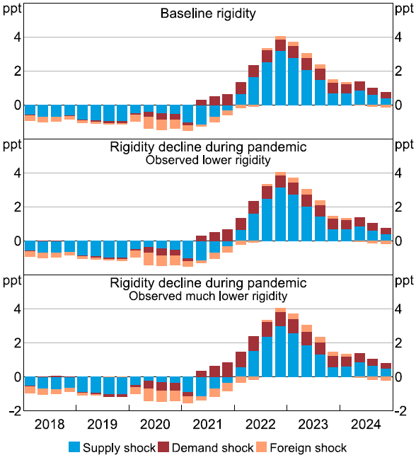
Notes: Supply shocks include mark-up, technology and labour supply shocks, and will capture some overseas shocks. Demand shocks include monetary policy, investment and consumption shocks. Foreign shocks include foreign demand and cost shocks.
Sources: ABS; Authors' calculations.
References
ABS (Australian Bureau of Statistics) (2018), ‘A Guide to the Consumer Price Index: 17th Series’, ABS website, available at <https://www.abs.gov.au/statistics/economy/price-indexes-and-inflation/guide-consumer-price-index-17th-series/latest-release#cite-window1>.
Adolfson M, S Laséen, J Lindé and LEO Svensson (2011), ‘Optimal Monetary Policy in an Operational Medium-sized DSGE Model’, Board of Governors of the Federal Reserve System, International Finance Discussion Paper No 1023.
Alvarez F, H Le Bihan and F Lippi (2016), ‘The Real Effects of Monetary Shocks in Sticky Price Models: A Sufficient Statistic Approach’, The American Economic Review, 106(10), pp 2817–2851.
Alvarez F, F Lippi and A Oskolkov (2022), ‘The Macroeconomics of Sticky Prices with Generalized Hazard Functions’, The Quarterly Journal of Economics, 137(2), pp 989–1038.
Auclert A, R Rigato, M Rognlie and L Straub (2024), ‘New Pricing Models, Same Old Phillips Curves?’, The Quarterly Journal of Economics, 139(1), pp 121–186.
Beckers B, J Hambur and T Williams (2023), ‘Estimating the Relative Contributions of Supply and Demand Drivers to Inflation in Australia’, RBA Bulletin, June.
Benigno P and GB Eggertsson (2023), ‘It's Baaack: The Surge in Inflation in the 2020s and the Return of the Non-linear Phillips Curve’, NBER Working Paper No 31197.
Bilyk O, M Khan and O Kostyshyna (2024), ‘Pricing Behaviour and Inflation during the COVID-19 Pandemic: Insights from Consumer Prices Microdata’, Bank of Canada Staff Analytical Note 2024-6.
Blanchard O and J Galí (2010), ‘Labor Markets and Monetary Policy: A New Keynesian Model with Unemployment’, American Economic Journal: Macroeconomics, 2(2), pp 1–30.
Blanco A, C Boar, CJ Jones and V Midrigan (2024a), ‘Non-linear Inflation Dynamics in Menu Cost Economies’, NBER Working Paper No 32094.
Blanco A, C Boar, CJ Jones and V Midrigan (2024b), ‘Nonlinear Dynamics in Menu Cost Economies? Evidence from U.S. Data’, NBER Working Paper No 32748.
Blanco A, C Boar, CJ Jones and V Midrigan (2024c), ‘The Inflation Accelerator’, NBER Working Paper No 32531, rev March 2025.
Cagliarini A, T Robinson and A Tran (2010), ‘Reconciling Microeconomic and Macroeconomic Estimates of Price Stickiness’, RBA Research Discussion Paper No 2010-01.
Calvo GA (1983), ‘Staggered Prices in a Utility-maximizing Framework’, Journal of Monetary Economics, 12(3), pp 383–398.
Cavallo A (2018), ‘Scraped Data and Sticky Prices’, The Review of Economics and Statistics, 100(1), pp 105–119.
Cavallo A, F Lippi and K Miyahara (2024), ‘Large Shocks Travel Fast’, The American Economic Review: Insights, 6(4), pp 558–574.
Cavallo A and R Rigobon (2016), ‘The Billion Prices Project: Using Online Prices for Measurement and Research’, The Journal of Economic Perspectives, 30(2), pp 151–178.
De Fiore F, B Mojon, D Rees and D Sandri (2023), ‘Monetary Policy Frameworks Away from the ELB’, BIS Working Paper No 1156.
Dedola L, E Gautier, A Nakov, S Santoro, E De Veirman, L Henkel and B Fagandini (2023), ‘Some Implications of Micro Price-setting Evidence for Inflation Dynamics and Monetary Transmission’, ECB Occasional Paper No 321.
Gagliardone L, M Gertler, S Lenzu and J Tielens (2025), ‘Micro and Macro Cost-Price Dynamics in Normal Times and during Inflation Surges’, NBER Working Paper No 33478, rev July 2025.
Gautier E, C Conflitti, D Enderle, L Fadejeva, A Grimaud, E Gutiérrez, V Jouvanceau, J-O Menz, A Paulus, P Petroulas, P Roldan-Blanco and E Wieland (2026), ‘Consumer Price Stickiness in the Euro Area during an Inflation Surge’, ECB Working Paper No 3181.
Gautier E, C Conflitti, RP Faber, B Fabo, L Fadejeva, V Jouvanceau, J-O Menz, T Messner, P Petroulas, P Roldan-Blanco, F Rumler, S Santoro, E Wieland and H Zimmer (2024), ‘New Facts on Consumer Price Rigidity in the Euro Area’, American Economic Journal: Macroeconomics, 16(4), pp 386–431.
Gelain P and P Lopez (2024), ‘Understanding Post-pandemic Surprises in Inflation and the Labor Market’, Federal Reserve Bank of Cleveland Economic Commentary No 2024-11.
Gibbs CG, J Hambur and G Nodari (2021), ‘Housing and Commodity Investment Booms in a Small Open Economy’, Economic Record, 97(317), pp 212–242.
Guimaraes B and KD Sheedy (2011), ‘Sales and Monetary Policy’, The American Economic Review, 101(2), pp 844–876.
Harding M, J Lindé and M Trabandt (2022), ‘Resolving the Missing Deflation Puzzle’, Journal of Monetary Economics, 126, pp 15–34.
Henkel LE Wieland, A Błażejowska, C Conflitti, B Fabo, L Fadejeva, J Jonckheere, P Karadi, P Macias, J-O Menz, P Seiler and K Szafranek (2023), ‘Price Setting during the Coronavirus (COVID-19) Pandemic’, European Central Bank Occasional Paper No 324.
Ilut C, R Valchev and N Vincent (2020), ‘Paralyzed by Fear: Rigid and Discrete Pricing under Demand Uncertainty’, Econometrica, 88(5), pp 1899–1938.
Karadi P, A Nakov, G Nuño, E Pastén and D Thaler (2024), ‘Strike while the Iron is Hot: Optimal Monetary Policy with a Nonlinear Phillips Curve’, BIS Working Paper No 1203, rev 7 August 2024.
Klein M, K Strömberg and O Tysklind (2024), ‘Inflation Dynamics in the High Inflation Period: Insights from Microdata’, Sveriges Riksbank Economic Commentary No 14.
Klenow PJ and BA Malin (2010), ‘Microeconomic Evidence on Price-setting’, in BM Friedman and M Woodford (eds), Handbook of Monetary Economics: Volume 3A, Handbooks in Economics, Elsevier, Amsterdam, pp 231–284.
Kryvtsov O and N Vincent (2021), ‘The Cyclicality of Sales and Aggregate Price Flexibility’, The Review of Economic Studies, 88(1), pp 334–377.
Lane PR (2024), ‘The 2021-2022 Inflation Surges and the Monetary Policy Response through the Lens of Macroeconomic Models’, SUERF Marjolin Lecture given at the 36th SUERF Colloquium ‘Inflation, Inflation Expectations, and Policy: New Perspectives’ hosted by Banca d'Italia, Rome, 18–19 November.
Lowe P and L Ellis (1997), ‘The Smoothing of Official Interest Rates’, in P Lowe (ed), Monetary Policy and Inflation Targeting, Proceedings of a Conference, Reserve Bank of Australia, Sydney, pp 286–312.
Maćkowiak B and F Smets (2008), ‘On Implications of Micro Price Data for Macro Models’, ECB Working Paper No 960.
Montag H and D Villar (2025), ‘Post-pandemic Price Flexibility in the U.S.: Evidence and Implications for Price Setting Models’, Board of Governors of the Federal Reserve System Finance and Economics Discussion Series No 2025-024.
Nakamura E and J Steinsson (2008), ‘Five Facts about Prices: A Reevaluation of Menu Cost Models’, The Quarterly Journal of Economics, 123(4), pp 1415–1464.
Roberts JM (1995), ‘New Keynesian Economics and the Phillips Curve’, Journal of Money, Credit and Banking, 27(4), pp 975–984.
Rotemberg JJ (1982), ‘Sticky Prices in the United States’, Journal of Political Economy, 90(6), pp 1187–1211.
Rotemberg JJ (1987), ‘The New Keynesian Microfoundations’, in S Fischer (ed), NBER Macroeconomics Annual 1987, 2, The MIT Press, Cambridge, pp 69–104.
Rudolf B and P Seiler (2022), ‘Price Setting before and during the Pandemic: Evidence from Swiss Consumer Prices’, ECB Working Paper No 2748.
Schmitt-Grohé S and M Uribe (2025), ‘Heterogeneous Downward Nominal Wage Rigidity: Foundations of a Nonlinear Phillips Curve’, Unpublished manuscript, Columbia University, 13 October.
Sutton M (2017), ‘The Average Size and Proportion of Price Changes in the CPI’, in ‘Consumer Price Index, Australia, September Quarter 2017’, ABS Cat No 6401.0, pp 12–21.
Taylor JB (1993), ‘Discretion versus Policy Rules in Practice’, Carnegie-Rochester Conference Series on Public Policy, 39, pp 195–214.
Turen J (2023), ‘State-dependent Attention and Pricing Decisions’, American Economic Journal: Macroeconomics, 15(2), pp 161–189.
Copyright and Disclaimer Notice
BLADE Disclaimer
The following Disclaimer Notice refers to data and graphs sourced from the Australian Bureau of Statistics' BLADE (Business Longitudinal Analysis Data Environment) database.
The results of these studies are based, in part, on data supplied to the ABS under the Taxation Administration Act 1953, A New Tax System (Australian Business Number) Act 1999, Australian Border Force Act 2015, Social Security (Administration) Act 1999, A New Tax System (Family Assistance) (Administration) Act 1999, Paid Parental Leave Act 2010 and/or the Student Assistance Act 1973. Such data may only be used for the purpose of administering the Census and Statistics Act 1905 or performance of functions of the ABS as set out in section 6 of the Australian Bureau of Statistics Act 1975. No individual information collected under the Census and Statistics Act 1905 is provided back to custodians for administrative or regulatory purposes. Any discussion of data limitations or weaknesses is in the context of using the data for statistical purposes and is not related to the ability of the data to support the Australian Taxation Office, Australian Business Register, Department of Social Services and/or Department of Home Affairs' core operational requirements.
Legislative requirements to ensure privacy and secrecy of these data have been followed. For access to MADIP and/or BLADE data under Section 16A of the ABS Act 1975 or enabled by section 15 of the Census and Statistics (Information Release and Access) Determination 2018, source data are de-identified and so data about specific individuals has not been viewed in conducting this analysis. In accordance with the Census and Statistics Act 1905, results have been treated where necessary to ensure that they are not likely to enable identification of a particular person or organisation.
Acknowledgements
Thanks to Erwan Gautier, Christopher Gibbs, Sarah Hunter, Matthias Klein, Kevin Lane and Claude Lopez for their helpful feedback on this work, and to seminar participants at the RBA, Bank for International Settlements, Bank of Korea, University of Melbourne, University of Queensland, University of Sydney, Australian National University and the 2025 e61/UNSW Macroeconomic Policy Workshop. Thanks to Omer Majeed for making significant contributions to the initial set-up and exploration of our dataset. The views expressed in this paper are those of the authors and should not be attributed to the Reserve Bank of Australia. Any errors are the sole responsibility of the authors.
Footnotes
Rotemberg pricing is another form of non-state-dependent pricing commonly used in macro models, where rigidity arises nonlinearly because firms face quadratic price adjustment costs (Rotemberg 1982). In log-linearised models, it results in identical predictions of pass-through as Calvo models, despite the different pricing mechanism. Nonlinear Phillips curves may arise through other mechanisms, such as the specific form of the demand function (Harding, Lindé and Trabandt 2022), and via labour market frictions (Benigno and Eggertsson 2023; Schmitt-Grohé and Uribe 2025). [1]
While these papers document a change in price-setting rigidity, they tend not to test which mechanism is driving firms to shift their behaviour (i.e. menu costs versus changing attention and frequency of price reviews). [2]
Items in the goods component of the CPI that are notably absent from the web-scraped dataset include food & non-alcoholic beverages, tobacco, new dwellings, motor vehicles and automotive fuel. [3]
These assumptions are standard in the web-scraped prices microdata literature, as well as in statistical agencies that collect online prices as a part of compiling official price indices. For example, see ‘Collecting prices for the CPI’ in ABS (2018). A further discussion of principles for selecting retail firms for web-scraping-based research can be found in Cavallo and Rigobon (2016). [4]
For contrasting views on the relevance of sales pricing to inflation dynamics and monetary policy analysis, see Guimaraes and Sheedy (2011) and Kryvtsov and Vincent (2021). [5]
This builds on the approach described in Gautier et al (2024). [6]
See Appendix B for figures showing how the distribution of the size of price changes has evolved over time. [7]
In general, there tend to be more price decreases than increases for advertised retail prices, and more increases than decreases for regular retail prices. This reflects that advertised prices include clearance sales while these are excluded from regular prices. [8]
An alternative would be the number of price changes each month, but due to irregular sampling frequency such measures may be biased. [9]
Where a ‘price spell’ is defined as the number of days between when a price is set and when it next changes. [10]
The results of our analysis were robust to an alternative assumption that the probability distribution underlying the present function was a Weibull distribution. [11]
To account for data collection gaps that could be misinterpreted as long price spells, we also test a specification that excludes price spells with gaps longer than 30 days between observations. While this adjustment affects the level of estimated rigidity, it does not materially alter the trend over time. [12]
We consider allowing baseline hazard rates to vary by item, but this proves computationally intensive given the size of the dataset. We also test a specification in which price spells are split across quarters, allowing hazard rates to reflect all periods spanned rather than just the start date. However, this approach produces volatile estimates that are sensitive to future data updates. For example, the addition of new data for 2024 could retroactively alter estimates for 2022 by changing the interpretation of spells spanning both years. Our preferred specification – anchoring hazard rates to the quarter or year in which a spell begins – offers greater stability and interpretability. [13]
We perform the analysis across all firms and products. We are limited from exploring heterogeneity across firm industries by privacy requirements. Future analysis could be done by CPI component if item-level categorisations are made available by the ABS. [14]
Detailed regression results are provided in Appendix C. [15]
Importantly, differences between empirical microdata and DSGE model-based calibrations of price rigidity do not necessarily imply that structural models are incorrectly specified. Calvo parameters in DSGE models are designed to capture aggregate price stickiness, which may reflect broader economic frictions and abstract from firm-level heterogeneity. For further discussion, see Maćkowiak and Smets (2008) and Cagliarini et al (2010). [16]
A theory of price rigidity based on firms' uncertainty about the competitive environment is developed in Ilut, Valchev and Vincent (2020). [17]
Our data includes some products (such as clothes and electronics) whose prices would typically be expected to decline steadily over their life span. It is possible that upward pressure on input costs for these products might result in firms slowing the frequency of price decreases, rather than increasing the frequency of changes. This would give the appearance that price rigidity was increasing alongside rising inflation, though the lower frequency of price changes would support rising inflation. To the extent that this is a factor, we expect that it will make the decline in rigidity in our dataset look more modest than it is. [18]
This model is described in detail in Gibbs, Hambur and Nodari (2021). [19]
A formal Chi-squared test of estimated survival analysis coefficients showed that coefficients in each year after 2019 were statistically different from the coefficient in 2019. [20]
See proof and discussion in Rotemberg (1987) and Roberts (1995). [21]
For this analysis, we abstract from the price indexation term and assume it remains unchanged. [22]
That said, we acknowledge that some prices, such as administered prices that are indexed and updated on a set schedule, are unlikely to have had changes in their price-setting frequency in the high-inflation period. [23]
We also test the impact of a positive 1 per cent domestic consumption (demand) shock on the price level under alternative price rigidities; in general, the results are similar to those following the cost-push shock, though of somewhat smaller magnitude. For example, accounting for the decline in price rigidity with a consumption shock results in a price level estimate around 2 to 20 per cent higher in the long run. [24]
It is also somewhat similar to the decomposition in Lane (2024), where European inflation outcomes are decomposed into those reflecting incorrect assumptions about exogenous variables like energy prices, and those that cannot be explained by incorrect assumptions. [25]
One limitation of this approach is that the recovered shocks prior to 2022 are based on lower rigidity assumptions, whereas our results in Section 5 suggest that rigidity may have been higher during the early pandemic period. This could introduce minor bias due to autoregressive shock dynamics, but we expect the impact to be second order. [26]
More precisely the target for inflation is the average rate, which is closer to 2.6 per cent. [27]
A decline in price rigidity also implies a lower welfare cost of inflation, which could justify placing less weight on inflation in the policy loss function. We test a variant of the exercise where the inflation weight is reduced by 30 per cent, consistent with the decline in the social cost of inflation implied by lower rigidity in simple DSGE models (e.g. Blanchard and Galí 2010). While this adjustment brings the optimal policy path closer to the baseline, we caution against over-interpreting the result. The RBA's DSGE model is more complex than the stylised frameworks used to derive such adjustments, and the calibration of the weight change may not be directly transferable. [28]
One weakness of the approach is that the times that we face lower rigidities are exactly those times where the shocks hitting the economy are extreme. That said, the exercise still provides a general sense of the change in trade-offs. [29]
Note that both coefficients decline in absolute terms, particularly the output coefficient. This reflects the fact that, under lower rigidity, monetary policy has a stronger effect on real interest rates. Given this, demand shocks – which do not involve a trade-off between inflation and output – can be addressed with smaller interest rate adjustments. [30]
An example might be two t-shirts in the same style that are different colours. [31]
These are likely to be lower bound estimates for a given item over the sample period, as in an practice items will regularly drop out of the sample as they are retired. [32]
Adjusting the time windows used to identify temporary and clearance sales has only minor effects on our results. [33]
As a robustness test, we run a version of the item-weighted yearly kernel distributions holding the firm sample fixed between 2019 and 2023. The measured shape of distributions is not significantly different, nor is the evolution of changes in distributions over time. That said, there is some variation in the height of various peaks in the distribution away from the centre. This suggests the need for caution in interpretating sales-related peaks; that is, the relative height of the peaks is affected by compositional change in which firms are sampled over time. [34]
For theoretical support, see Alvarez, Lippi and Oskolkov (2022) and Cavallo et al (2024). For empirical evidence, refer to the recent studies cited in Section 2. [35]