RDP 2025-08: Ageing and Economic Growth in China 2. Data, Methodology and Identification
November 2025
2.1 Data
To apply this methodology for China, I collect province-level population counts by age from China's National Bureau of Statistics (NBS) census tabulations for the 1990, 2000, 2010 and 2020 censuses.[3] The 1982 census – the first of China's ‘reform and opening’ period – does not provide this tabulation publicly, so I estimate provincial population by age for 1982 using the IPUMS International 1 per cent sample of the microdata for the 1982 census (Ruggles et al 2024).[4] I collect NBS data on GDP per capita by province for 1990, 2000, 2010 and 2020 from the CEIC database.
I also collect the province-level proportion of employment by industry from the census for 1990, 2000 and 2010 for use as a time-varying control in the robustness checks described in Section 3.1.1. These employment figures are available from the 2000 and 2010 NBS tabulations, with a series of industry classifications that I summarise into four categories: agriculture, mining, manufacturing and other. As the 1990 Census industry-by-province employment is not available in the NBS tabulation, I use the IPUMS International 1 per cent microdata sample from the 1990 census to calculate the proportion of employment.
2.2 Methodology
As in MMP, I estimate the following regression of decadal log differences in GDP per capita on decadal log differences in the proportion of population aged over 60. In the regression, notation p indicates province, t is year, X is a set of time-varying control variables and is time fixed effects.[5] A is population aged over 60, and N is total population aged over 20.
I instrument the log differences in proportion of population over 60 with the predetermined component of ageing, using what MMP call a 20-year lag length – that is, I use the population structure at t −10, where t is the beginning year of the decade for which the effect on GDP growth is being estimated. The instrument is generated as:
where
and
Put plainly, for the 20-year lag instrument I calculate the predicted population over 60 at time t and t +10 by first multiplying the population in each province at time t −10 by the national level survival rate between t −10 to t and t +10, respectively, for the relevant age cohort. The national survival rates are calculated by taking the ratio of the total national age cohort at time t and t +10 compared to the size of the relevant age cohort at time t −10 (for example, the size of the 40–45 age cohort at time t on the size of the 30–35 cohort at time t −10 ). I then take the ratio of the predicted population aged over 60 at time t and t +10 and predicted total population aged over 20 for each province and period. The instrument is the log of the predicted population ratio over 60 at time t +10 subtracting the log of the predicted population ratio over 60 at time t.
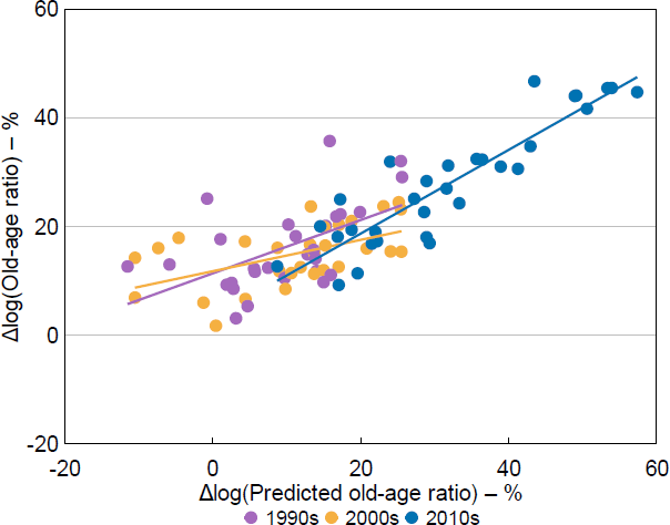
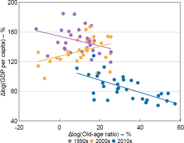
I illustrate the relationship between the instrument and actual ageing in Figure 5, between actual ageing and GDP per capita growth in Figure 6, and between the instrument and GDP per capita growth in Figure 7. Each dot represents a province, and the colour indicates the decade of the observation. Appendix A also includes map representations of the ageing data.
Sources: Author's calculations; CEIC Data; National Bureau of Statistics of China.
Sources: Author's calculations; CEIC Data; National Bureau of Statistics of China.
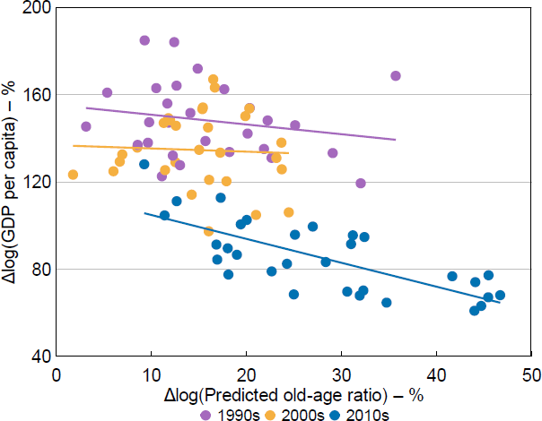
Sources: Author's calculations; CEIC Data; National Bureau of Statistics of China.
2.3 Identification
To meet the assumptions necessary for a valid instrumental variable, the instrument must be relevant, exogenous, and meet the exclusion assumption. The relevance assumption requires the instrument (predetermined component of the increase in population over 60) to be correlated with the key regressor (increase in population over 60). This would logically be true absent extreme levels of internal migration, and a weak instrument test rejects the hypothesis that the instrument is irrelevant.[6]
The exogeneity assumption requires that the instrument be uncorrelated with the error term . The exclusion restriction requires that the instrument does not affect economic growth except for through the instrumented variable: the actual change in the old-age ratio. The exogeneity and exclusion assumptions together require that a province's ‘past age structure affects future changes in economic outcomes only by affecting its subsequently realized age structure, and not through any other channel’ (MMP, p 313). For example, the predicted change in population should not be systematically correlated with exogenous shocks based on industry structure such as trade shocks. As another example, suppose slower growth in a region due to a negative demand shock induces higher mortality in the region, spuriously increasing the correlation between growth and the old-age ratio. Predicted ageing in the population should be uncorrelated with that negative demand shock.
A threat to the instrumental variable assumptions is if there is significant migration in a way that was systematically correlated with migrants' expectations for the province's economic growth between 10- and 20-years' time (not just the level of GDP per capita of the province at that time). While migrants undoubtedly make migration decisions on the basis of expectations for their labour market outcomes, which are in turn determined by the industry structure and growth prospects of the target province, until 2000 internal migrants in China overwhelmingly tended to be aged between 16 and 44 (NBS, UNFPA and UNICEF 2018), which is a somewhat less important cohort for identification in this model, as discussed below.
For the exogeneity assumption to hold, there also cannot be persistent shocks in the past that affect both predicted ageing (i.e. the population structure in the past) and growth in the future. While it is likely that factors such as natural resource allocation and the structural features of the Chinese political and economic system in the mid-20th century affect both population structures in the late 20th century and the level of development of a given province, it is less clear that these factors would affect the growth rate in a particular decade in the future. To illustrate the distinction, while GDP per capita in levels is highly correlated among provinces from decade to decade, the correlation between provincial GDP per capita growth in the 1990s and in the 2010s is actually slightly negative.[7] That is, even if households can, on average, predict provincial growth in the next decade, they may not necessarily correctly predict growth in the decade following that. To further account for potential identification issues, I explore the robustness of the estimates in Section 3 by stretching back the lag of the instrument to t – 20 and t −30. Increasing the time difference between the census used to generate the instrument and the observations in question should reduce the likelihood of expectations or persistent shocks playing a biasing role.
The MMP instrument is in spirit a Bartik, or ‘shift-share’ type instrument. The construction of these type of instruments can make interpretation of the identifying assumptions difficult. In this ‘shift-share’ instrument, the ‘share’ is the proportion of provincial population in each age cohort at t −10, and the ‘shift’ is the national-level cohort survival rates. To expound on where the identification originates in the MPP instrument, I follow Goldsmith-Pinkham, Sorkin and Swift (2020) in decomposing the Rotemberg weights of the equivalent GMM estimator with age cohort-by-province shares as instruments. These weights are interpretable as showing the components of the Bartik instrument to which the estimates are most sensitive to misspecification. That is, greater Rotemberg weights for an age cohort imply that the identification of the instrumental variables is more reliant on the variation in the proportion of population in that cohort between provinces.
The population cohort shares at t −10 which have the largest (absolute) Rotemberg weights are those cohorts which age into the over-50 category by time t, followed by the birth cohorts in the decade prior to t −10, which will age into the denominator of the old-age ratio (all people aged over 20) (Table 1). Put simply, the estimation approach can be thought of as mostly comparing the GDP per capita growth rates for t to t +10 between provinces with larger and smaller populations aged over 50 at t −10, as well as higher and lower birth rates between t −20 and t −10. The size of the population over 50 at t −10 would be determined by the province birth rate at time t −60 and earlier, and by migration decisions of people in that age cohort from anywhere between t −70 and t −10.
| Age cohort | Cohort share of population(a) | |
|---|---|---|
| 50+ | 0.375 | 0.187 |
| 0–9 | 0.296 | 0.145 |
| 40–49 | 0.176 | 0.135 |
| 10–39 | 0.154 | 0.524 |
|
Notes: Unlike in the canonical Bartik instrument where Rotemberg weights are usually positive, in this instrument some weights are negative by construction (increasing in size of cohorts which are only in the denominator of the old-age ratio subtracts from the ratio). I therefore present the weights as absolute weight on sum of absolute weights to give a clearer interpretation of cohort importance. (a) Average across provinces and years. |
||
Footnotes
The main regressions include all provincial-level administrative units except for Chongqing and Sichuan (since the two were split in 1997) and Hainan (which was split from Guangdong, a considerably more populous province, in 1988). [3]
Specifically, I calculate the proportion of the population by age in each province from the 1 per cent sample of the microdata and then multiply by the provincial aggregate population counts reported in the NBS census tabulation to construct aggregate provincial population by age. This induces a slight (but likely random) error in the age-by-province population counts for 1982. The 1 per cent sample includes around 11 million people. [4]
The time-varying controls in the baseline results are whether or not the province is coastal, and the coastal variable with a time interaction. I include these geographic controls to account for the possibility that the significant increase in trade after China's accession to the World Trade Organization (WTO) in the 2000s, which would accrue mainly to the coastal provinces, could affect the results. [5]
An F-test returns an F-statistic of 71 for the instrument, well above the rule of thumb that the F-statistic should be above 10 to avoid a weak instrument (Staiger and Stock 1997). See Appendix A. [6]
See Appendix A. This pattern would be expected if less-developed provinces are expected to catch up to the GDP levels of more-developed provinces over time. Between the 2000s and 2010s on the other hand, this correlation is positive. [7]