RDP 2013-10: Stochastic Terms of Trade Volatility in Small Open Economies 3. Estimating the Law of Motion for the Terms of Trade
August 2013 – ISSN 1320-7229 (Print), ISSN 1448-5109 (Online)
- Download the Paper 1.06MB
In this section, we estimate the empirical process for the terms of trade for six small open economies: Australia, Brazil, Canada, Mexico, New Zealand and South Africa. We select these countries based on two criteria. First, we focus on commodity-producing small open economies whose terms of trade are both volatile and plausibly exogenous to domestic economic developments. Second, we require countries to have reasonably long time series data for the terms of trade and other macroeconomic variables.
To support our contention that the terms of trade are exogenous, Table 1 provides descriptive statistics about the size and export composition of each economy. The six economies each account for a small share of world GDP and merchandise trade. This suggests that economic developments within these countries are unlikely to have a substantial effect on world economic activity. Moreover, the exports of these countries are geared towards agriculture, fuels and mining – that is, commodities – with these goods accounting for more than 50 per cent of merchandise export values for each country, except Mexico.[1] Commodities tend to be less differentiated, and more substitutable, than manufactured goods and commodity producers generally have less pricing power on world markets.[2] Further evidence to support our contention comes from the numerous studies that have used statistical techniques to examine the exogeneity of the terms of trade for small open economies. For example, using Granger causality tests, Mendoza (1995) and Broda (2004) conclude that the terms of trade is exogenous for a large sample of small open economies, including Brazil, Canada and Mexico.
| Share of world merchandise exports |
Export composition | |||
|---|---|---|---|---|
| Food items and agricultural raw materials |
Fuels, ores and metals |
Manufactured goods |
||
| Australia | 1.4 | 13.1 | 69.2 | 12.8 |
| Brazil | 1.3 | 34.8 | 29.5 | 35.8 |
| Canada | 2.5 | 13.5 | 35.6 | 47.8 |
| Mexico | 2.0 | 6.3 | 18.7 | 74.5 |
| New Zealand | 0.2 | 63.3 | 10.1 | 22.9 |
| South Africa | 0.6 | 10.5 | 47.4 | 39.2 |
|
Source: UNCTAD (2011) |
||||
3.1 Estimation
For each country, we specify that the terms of trade, qt, follow an AR(1) process described by:

where uq,t are normally distributed shocks with mean zero and unit variance.[3] The log of the standard deviation of the terms of trade shocks, σq,t, varies over time, according to an AR(1) process:

where uσ,t are normally distributed shocks with mean zero and unit variance. To emphasise, innovations to uq,t alter the level of the terms of trade. In contrast, innovations to uσ,t alter the magnitude of shocks to the terms of trade, with no direct effect on its level. We refer to these as volatility shocks. The parameter σq is the log of the mean standard deviation of terms of trade shocks, while ηq is the standard deviation of shocks to the volatility of the terms of trade. The parameter ρq controls the persistence of shocks to the level of the terms of trade, while ρσ controls the persistence of terms of trade volatility shocks. Throughout, we assume that uq,t and uσ,t are independent of each other.
Equations (1) and (2) represent a standard stochastic volatility model. Inference in these models is challenging because of the presence of two innovations, one to the level of the terms of trade and one to its volatility, that enter the model in a non-linear manner. To overcome this issue, we follow Fernández-Villaverde et al (2011) and use a sequential Markov chain Monte Carlo filter, also known as a particle filter, that allows us to evaluate the likelihood of the model using simulation methods. We estimate the model using a Bayesian approach that combines prior information with information that can be extracted from the data. For presentational ease, we confine the technical details of the estimation procedure to Appendix C.
Other methods of modeling time-varying volatility processes, including Markov switching models and GARCH models, also exist. Although these methods have advantages in other contexts, we do not believe that they provide a satisfactory description of terms of trade volatility. For example, a GARCH model does not sharply distinguish between innovations to the level of the terms of trade and its volatility. High levels of volatility are triggered only by large innovations to the terms of trade. In contrast, our methodology allows changes in the volatility of the terms of trade to occur independently of innovations to the level of the terms of trade. Nonetheless, for comparison Appendix D shows the results when we estimate the terms of trade processes using a GARCH model. A Markov switching model would require us to restrict the number of potential realisations of terms of trade volatility in a way that seems inconsistent with the patterns in Figure 1.
3.2 Data
The terms of trade for each country are measured quarterly, and defined as the ratio of the export price deflator to the import price deflator and sourced from national statistical agencies.[4] As we wish to estimate changes over time in the variance of the terms of trade, we require our data to be stationary. It is not clear whether real commodity prices (which drive the terms of trade for the countries in our sample) are stationary. Previous studies by Powell (1991), Cashin, Liang and McDermott (2000) and Lee, List and Strazicich (2006), among others, have concluded that real commodity prices are stationary. Others, including Kim et al (2003), Newbold, Pfaffenzeller and Rayner (2005) and Maslyuk and Smyth (2008) have found that they are not.
In light of the disagreement in the literature, we adopt a compromise approach and detrend our data using a band-pass filter that excludes cycles of longer than 30 years. This preserves all but the lowest frequency movements in the terms of trade for each country while ensuring that the data are stationary.[5]
3.3 Priors
Table 2 reports our priors for the parameters of the terms of trade process. For the persistence parameters, ρq and ρσ, we impose a Beta prior with mean of 0.9 and standard deviation of 0.1. The shape of this prior restricts the value of these parameters to lie between 0 and 1, consistent with economic theory. For the log of the mean standard deviation of terms of trade shocks, σq, we impose a Normal prior. For each country, we set the mean of this prior equal to the OLS estimate of this parameter calculated assuming an AR(1) process for the terms of trade without stochastic volatility. For the standard deviation of terms of trade volatility shocks, ηq, we use a truncated Normal prior to ensure that this parameter is positive. We experimented with alternative priors and found that these had very little impact on our results.
| Parameter | ρq | σq | ρσ | ηq |
|---|---|---|---|---|
| Prior | β (0.9,0.1) |
 ( (
 ,0.4) ,0.4) |
β(0.9,0.1) |
+(0.5,0.3) |
Note: β,
and
 stand for Beta, Normal and
truncated Normal distributions stand for Beta, Normal and
truncated Normal distributions |
||||
3.4 Posterior Estimates
Table 3 reports the posterior medians of the parameter estimates and associated confidence bands. The first row shows the posterior estimates of ρq, the persistence of the terms of trade processes. This parameter lies above 0.9 for all countries except for South Africa, indicating that shocks to the terms of trade for these countries tend to be highly persistent.
| Australia | Brazil | Canada | Mexico | New Zealand | South Africa | |
|---|---|---|---|---|---|---|
| ρq | 0.93 | 0.96 | 0.90 | 0.92 | 0.96 | 0.81 |
| (0.88, 0.98) | (0.90, 0.99) | (0.85, 0.95) | (0.87, 0.97) | (0.89, 0.97) | (0.73, 0.86) | |
| σq | −3.65 | −3.22 | −4.40 | −3.43 | −3.48 | −3.30 |
| (−4.16,−3.03) | (−3.74,−2.57) | (−4.74,−4.04) | (−3.78,−3.03) | (−3.93,−2.90) | (−3.81,−2.76) | |
| ρσ | 0.94 | 0.92 | 0.85 | 0.85 | 0.93 | 0.97 |
| (0.83, 0.99) | (0.79, 1.00) | (0.57, 0.98) | (0.64, 0.94) | (0.84, 1.00) | (0.85, 1.00) | |
| ηq | 0.21 | 0.21 | 0.26 | 0.38 | 0.13 | 0.10 |
| (0.12,0.33) | (0.11,0.36) | (0.13,0.48) | (0.25, 0.54) | (0.07, 0.23) | (0.05, 0.23) | |
| Note: 95 per cent credible sets in parantheses | ||||||
The parameter estimates for σq reveal substantial differences in the average size of shocks to the terms of trade between countries. Converting the parameters into standard deviations, the results suggest that the magnitude of the average terms of trade shock varies from around 1.2 per cent for Canada to 4.0 per cent for Brazil.[6] The estimates for ρσ indicate that shocks to the volatility of the terms of trade are highly persistent for Australia, Brazil, New Zealand and South Africa, but somewhat less so for Canada and Mexico.
The final row of Table 3 confirms that the magnitude of shocks to the volatility of the terms of trade differs across countries. Of the countries in our sample, Mexico has tended to experience the largest volatility shocks, while New Zealand and South Africa have experienced the smallest. To put these numbers in context, a one standard deviation shock to uσ,t increases the standard deviation of terms of trade shocks in Mexico from 3.2 per cent to 4.7 per cent and in South Africa from 3.7 per cent to 4.1 per cent.
To give a sharper insight into what our results imply for time-variation in terms of trade volatility, Figure 2 shows the model's estimates of the evolution of the standard deviations of terms of trade shocks for each country. The average level of volatility is higher for Brazil and Mexico than for the other countries in the sample, reflecting the fact that these countries have typically experienced larger terms of trade shocks. The changes in the level are also greatest for Mexico, as that country has experienced the largest shocks to the volatility of its terms of trade. In contrast, the standard deviation of shocks to Canada's terms of trade has typically been small and stable over time, at least compared to those experienced by other commodity exporters. The experiences of Australia, New Zealand and South Africa lie somewhere in between those of Canada and the Latin American countries. These economies have typically experienced large terms of trade shocks, with an average standard deviation of around 3 per cent. They have also experienced periods of heightened volatility, although not to the same extent as countries like Brazil and Mexico.
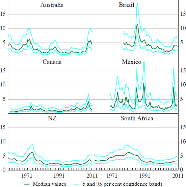
Notes:
Median values of exp ( ) where are the estimated volatilities
conditional on all information, calculated using the particle smoother
) where are the estimated volatilities
conditional on all information, calculated using the particle smoother
The patterns of volatility suggested by Figure 2 broadly conform to our understanding of macroeconomic developments over recent decades. For example, the average magnitudes of terms of trade shocks increased in most countries during the mid 1970s, mid 1980s and late 2000s, while the 1990s was generally a period of low terms of trade volatility.
In sum, our results indicate that the volatility of shocks to the terms of trade for small open economy commodity producers varies over time. Historically, the variation has been largest for Latin American countries such as Brazil and Mexico, where the standard deviation of terms of trade shocks has at times increased from an average level of around 3 per cent to over 10 per cent. But countries like Australia, New Zealand and South Africa have also experienced shocks that have increased the standard deviation of their terms of trade shocks from 2 per cent to around 6 per cent.
Footnotes
Even for Mexico, petroleum is the largest single export good at the three digit SITC 3 level, accounting for almost 12 per cent of total exports in 2010. Moreover, commodities accounted for the bulk of Mexico's exports in the early part of our sample, before the expansion of manufacturing exports that accompanied Mexico's trade liberalisation in 1986 and entry into NAFTA in 1994 (Moreno-Brid, Santamaría and Rivas Valdivia 2005). [1]
While this is not strictly true for all commodity producers, such as large oil producers for example, it seems reasonable for the countries in our sample. [2]
Our estimation procedure requires stationary data. We discuss the transformations that we make to ensure that our terms of trade series are stationary in the Data section below. [3]
Appendix A includes a full list of data sources and descriptions. [4]
We also estimated the models with HP-filtered data (see Appendix B for the results). The choice of detrending method has some effect on the estimated persistence of terms of trade shocks, but relatively little impact on the estimated magnitude of shocks to the terms of trade or the volatility processes. Appendix A provides figures (A1 and A2) of the terms of trade for each country in raw and filtered form to illustrate the effects of filtering methods on the underlying series. [5]
Recall, that the standard deviation of shocks to the terms of trade is equal to exp (σq). [6]