RDP 2011-01: Estimating Inflation Expectations with a Limited Number of Inflation-indexed Bonds 3. Data and Model Implementation
March 2011
- Download the Paper 480KB
3.1 Data
Four types of data are used in this analysis: nominal zero-coupon bond yields derived from nominal Australian Commonwealth Government bonds; Australian Commonwealth Government inflation-indexed bond yields; inflation forecasts from Consensus Economics; and historical inflation.
Nominal zero-coupon bond yields are estimated using the approach of Finlay and Chambers
(2009). These nominal yields correspond to  and are used in computing our function H1(xt) from
Equation (6). Note that the Australian nominal yield curve has a maximum maturity
of roughly 12 years. We extrapolate nominal yields beyond this by assuming
that the nominal and real yield curves have the same slope. This allows us
to utilise the prices of all inflation-indexed bonds, which have maturities
of up to 24 years (in practice the slope of the real yield curve beyond 12
years is very flat, so that if we instead hold the nominal yield curve constant
beyond 12 years we obtain virtually identical results).
and are used in computing our function H1(xt) from
Equation (6). Note that the Australian nominal yield curve has a maximum maturity
of roughly 12 years. We extrapolate nominal yields beyond this by assuming
that the nominal and real yield curves have the same slope. This allows us
to utilise the prices of all inflation-indexed bonds, which have maturities
of up to 24 years (in practice the slope of the real yield curve beyond 12
years is very flat, so that if we instead hold the nominal yield curve constant
beyond 12 years we obtain virtually identical results).
We calculate the real prices of inflation-indexed bonds using yield
data.[6]
Our sample runs from July 1992 to December 2010, with the available data sampled
at monthly intervals up to June 1994 and weekly intervals thereafter. Bonds
with less than one year remaining to maturity are excluded. By comparing these
computed inflation-indexed bond prices, which form the  in Equation (6), with our
function H1(xt), we are able to estimate the latent
factors. We assume that the standard deviation of the bond price measurement
error is
4 basis points. This is motivated by market liaison which suggests that,
excluding periods of market volatility, the bid-ask spread has stayed relatively
constant over the period considered, at around 8 basis points. Some descriptive
statistics for nominal and inflation-indexed bonds are given in Table 1.
in Equation (6), with our
function H1(xt), we are able to estimate the latent
factors. We assume that the standard deviation of the bond price measurement
error is
4 basis points. This is motivated by market liaison which suggests that,
excluding periods of market volatility, the bid-ask spread has stayed relatively
constant over the period considered, at around 8 basis points. Some descriptive
statistics for nominal and inflation-indexed bonds are given in Table 1.
| Time period | |||||
|---|---|---|---|---|---|
| Statistic | 1992–1995 | 1996–2000 | 2001–2005 | 2006–2010 | |
| Number of bonds: | nominal | 12–19 | 12–19 | 8–12 | 8–14 |
| inflation-indexed | 3–5 | 4–5 | 3–4 | 2–4 | |
| Maximum tenor: | nominal | 11–13 | 11–13 | 11–13 | 11–14 |
| inflation-indexed | 13–21 | 19–24 | 15–20 | 11–20 | |
| Average outstanding: | nominal | 49.5 | 70.2 | 50.1 | 69.5 |
| inflation-indexed | 2.1 | 5.0 | 6.5 | 7.1 | |
| Notes: Tenor in years; outstandings in billions; only bonds with at least one year to maturity are included | |||||
Note that inflation-indexed bonds are relatively illiquid, especially in comparison to nominal bonds.[7] Therefore, inflation-indexed bond yields potentially incorporate liquidity premia, which could bias our results. As discussed we use inflation forecasts as a measure of inflation expectations. These forecasts serve to tie down inflation expectations, and as such we implicitly assume that liquidity premia are included in our measure of risk premia. We also assume that the existence of liquidity premia causes a level shift in estimated risk premia but does not greatly bias the estimated changes in risk premia.[8]
The inflation forecasts are taken from Consensus Economics. We use three types of forecast:
- Monthly forecasts of the average percentage change in CPI over the current and the subsequent year.
- Quarterly forecasts of the year-on-year percentage change in the CPI for 7 or 8 quarters in the future.
- Biannual forecasts of the year-on-year percentage change in the CPI for each of the next 5 years, as well as from 5 years in the future to 10 years in the future.
We use the function H2(xt) to relate these inflation forecasts to the latent factors, and use the past forecasting performance of the inflation forecasts relative to realised inflation to calibrate the standard deviation of the measurement errors.
Historical inflation enters the model in the form of It,Δ from Section 2.3, but otherwise is not used in estimation. This is because the fundamental variable being modelled is the current instantaneous inflation rate. Given the inflation law of motion (implicitly defined by Equations (2) to (4)), inflation expectations and inflation-indexed bond prices are affected by current inflation and so can inform our estimation. By contrast, the published inflation rate is always ‘old news’ from the perspective of our model and so has nothing direct to say about current instantaneous inflation.[9]
3.2 The Kalman Filter and Maximum Likelihood Estimation
We use the Kalman filter to estimate the three latent factors using data on bond prices and inflation forecasts. The Kalman filter can estimate the state of a dynamic system from noisy observations. It does this by using information about how the state evolves over time, as summarised by the state equation, and relating the state to noisy observations using the measurement equation. In our case, the latent factors constitute the state of the system and our bond prices and forecast data the noisy observations. From the latent factors we are able to make inferences about inflation expectations and inflation risk premia.
The standard Kalman filter was developed for a linear system. Although our state equation (given by Equation (B1)) is linear, our measurement equations, using H1(xt) and H2(xt) as derived in Sections 2.3 and 2.4, are not. This is because we work with coupon-bearing bond prices instead of zero-coupon yields. We overcome this problem by using a central difference Kalman filter, which is a type of non-linear Kalman filter.[10]
The approximate log-likelihood is evaluated using the forecast errors of the Kalman
filter. If we denote the Kalman filter's forecast of the data at time t by 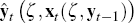 ,
which depends on the parameters (ζ) and the latent factors (xt(ζ,
yt−1)), which in turn depend on the parameters and
the data observed up to time t − 1 (yt−1),
then the approximate log-likelihood is given by
,
which depends on the parameters (ζ) and the latent factors (xt(ζ,
yt−1)), which in turn depend on the parameters and
the data observed up to time t − 1 (yt−1),
then the approximate log-likelihood is given by
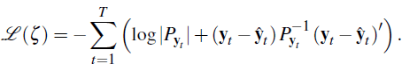
Here the estimated covariance matrix of the forecast data is denoted by  .[11] In the
model the parameters are given by
.[11] In the
model the parameters are given by 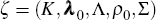 .
.
We numerically optimise the log-likelihood function to obtain parameter estimates. From the parameter estimates, we use the Kalman filter to obtain estimates of the latent factors.
3.3 Calculation of Model Estimates
For a given set of model parameters and latent factors, we can calculate inflation forward rates, expected future inflation rates and inflation risk premia.
In Appendix B we show that the expected future inflation rate at time t for time t + τ can be expressed as
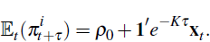
The inflation forward rate at time t for time  , is the rate of inflation at time t
+ τ implied by market prices of nominal and inflation-indexed
bonds trading at time t. As bond prices incorporate inflation risk,
so does the inflation forward rate. In our model the inflation forward rate
is given by
, is the rate of inflation at time t
+ τ implied by market prices of nominal and inflation-indexed
bonds trading at time t. As bond prices incorporate inflation risk,
so does the inflation forward rate. In our model the inflation forward rate
is given by
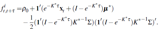
See Appendix B for details on the above and definitions of K* and μ*.
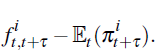
The inflation risk premium is given by the difference between the inflation forward rate, which incorporates risk aversion, and the expected future inflation rate, which is free of risk aversion. The inflation risk premium at time t for time t + τ is given by
Footnotes
Available from statistical table F16. [6]
Average yearly turnover between 2003/04 and 2007/08 was roughly $340 billion for nominal Government bonds and $15 billion for inflation-indexed bonds, which equates to a turnover ratio of around 7 for nominal bonds and 2½ for inflation-indexed bonds (see AFMA 2008). [7]
Inflation swaps are now far more liquid than inflation-indexed bonds and may provide alternative data for use in estimating inflation expectations at some point in the future. Currently, however, there is not a sufficiently long time series of inflation swap data to use for this purpose. [8]
Note that our model is set in continuous time; data are sampled discretely but all
quantities, for example the inflation law of motion as well as inflation
yields and expectations, evolve continuously.  from Equation (2) is the current instantaneous inflation rate, not a 1-month or
1-quarter rate.
[9]
from Equation (2) is the current instantaneous inflation rate, not a 1-month or
1-quarter rate.
[9]
See Appendix C for more detail on the central difference Kalman filter. [10]
In actual estimation we exclude the first six months of data from the likelihood calculation to allow ‘burn in’ time for the Kalman filter. [11]