RDP 8906: A Random Walk Around the $A: Expectations, Risk, Interest Rates and Consequences for External Imbalance Appendix B

This appendix examines the statistical properties of the exchange rates in Datasets A and B, including the conditional variance, covariance and skewness of the exchange rates. We provide a summary of our findings – further details are given in Smith (1989b).

For all the exchange rates in the two datasets we establish the following results. Using Perron and Phillips (1987) tests, we accept the null hypothesis that the log of the spot exchange rate at a one week interval (Dataset A) and one day interval (Dataset B) has no significant time trend but requires, at least, one unit difference to be stationary. Using Augmented Dickey-Fuller (1979) tests, we reject the hypothesis that the log exchange rate requires a second unit difference to be stationary. Thus, over the sample periods, these tests do not reject the hypothesis that each exchange rate follows a random walk with no drift.

The conditional variance of log changes in the spot exchange rate is successively modelled as autoregressive conditional heteroscedasticity [ARCH] (Engle, 1982), generalised ARCH [GARCH] (Bollerslev, 1986) and exponential GARCH [EGARCH] (Nelson, 1988). An ARCH(5) model is fitted to both datasets, and evidence for ARCH is found – although the explanatory power of the models is low. A GARCH(1,1) model is then fitted to both datasets, and the likelihood function shows this model to be far superior to the ARCH model. These two models impose a symmetrical distribution for the estimated conditional variance, while the EGARCH model does not. Given the significant skewness reported in section V, we expected to find evidence of EGARCH. In almost all cases, the parameter point estimates in our EGARCH model imply that there is greater volatility in the immediate aftermath of a fall in the $A than in the immediate aftermath of a rise. Unfortunately, the standard errors of the estimates are so large that this asymmetry is not statistically significant.

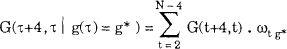
Rather than quote all the parameter estimates for each of the models, Figure 10 shows non-parametric estimates of the variance, skewness and two covariances for four-weekly changes in s[$US/$A], conditional on the change in s[$US/$A] over the previous week. We established that conditioning on the change in s[$US/$A] over the previous week provided more variability in the estimates than conditioning on the change in s[$US/$A] over the previous four weeks. Define s_t − s_{t − 1} = g(t), and imagine a variable G(t+4,t) defined in terms of exchange rates at times t and t+4 (e.g., G(t+4,t) = [s_{t + 4} − s_t]² or G(t+4,t) = [s_{t + 4} − s_t]³). With a sample s_t, t = 1,…,N, the non-parametric estimator of G(τ+4,τ) conditional on g(τ) = g^* is

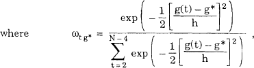
and h = σ_g. (N − 5)^−1/5 and σ_g is the standard error of the observations g(t), t = 2,…,N − 4. This non-parametric estimator is very similar to one suggested by Pagan and Schwert (1989).^[43] Figure 10 shows conditional estimates of (s_{t + 4}[$US/$A] − s_t[$US/$A])², (s_{t + 4}[$US/$A] − s_t[$US/$A])³, (s_{t + 4}[$US/$A] − s_t[$US/$A]).(s_{t + 4}[$US/$¥] − s_t[$US/$¥]) and (s_{t + 4}[$US/$A] − s_t[$US/$A]).(s_{t + 4}[$US/DM] − s_t[$US/DM]) based on Dataset A from Jan, 84 to Apr, 89. The third and fourth of these estimators correspond to covariances provided the expected change in the exchange rate over four weeks is zero, which is a good approximation. The unconditional sample estimates of the four variables above are, respectively, 12.63×10⁻⁴, −47.91×10⁻⁴, 2.30×10⁻⁴ and 2.46×10⁻⁴.

Within the sample, Figure 10 shows that the behaviour of the exchange rate over the next four weeks depends to a considerable extent on its movement in the previous week.^[44] Based on this figure, the risk premium required by a US investor after a fall of the $A of between 4% and 5% in the previous week should be substantial (using equation (10) and assuming a portfolio share in Australia of 0.02 as well as 0.10 in other foreign countries in the proportions used in the text, the risk premium is 0.5% p.a.). But, both this analysis and the analysis summarized above based on parametric approaches (ARCH, GARCH and EGARCH) suggest that the conditional moments of the change in the exchange rate over the next four weeks only depend on the exchange rate over the previous few weeks (probably no more than three weeks). As a consequence, these results do not undermine the conclusions reached in section III of the text. On average over extended periods (several weeks or several months), the risk premium which a utility maximizing US consumer-investor should demand for holding short-term nominal Australian assets seems to be negliglible – compared, for example, to the average short-term real interest differential between Australia and the US from late 84.

Footnotes

To deal with the problem of outliers in the g(τ) data, Pagan and Schwert (1989) suggest a slightly different estimate. We deal with this problem in a different way: after ordering the g(τ) sample from the most negative to the most positive, we only estimate G(τ+4,τ) for g^* values between the fifth smallest value of g(τ) and the fifth largest value of g(τ). [43]

However, the results of Pagan and Schwert (1989) suggest that, out of sample, the predictive capacity implied by the Figure is probably substantially overstated. [44]