RDP 8611: The Effectiveness of Fiscal Policy in an Economy with Anticipatory Wage Contracts 4. A Model of Debt and Money Finance with Flexible Prices

The previous model permitted only money finance of fiscal deficits. This meant that fiscal policy would have real effects only when output had suffered from an exogenous supply shock. When the government can also issue debt, fiscal policy can shock the real and the financial system out of a steady state.

The model can be reduced to three independent equations in and . Choosing the last three and summarising the model from (3)–(7), (10)'–(11)' and (12)–(14), we get

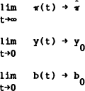
with the boundary conditions

Taking the determinant of the transition matrix in (28), one gets

Since there are two predetermined variables, y and b, in this model, we need two stable eigenvalues (that have negative real parts), and , and one stable one, S⁺. The product of these is Δ and must be positive if a saddlepath is to exist. Δ will be positive if t is sufficiently large. A sufficient condition is that , which means that the income tax rate must exceed the ratio of debt service to output. This condition will easily be met in a modern economy. The necessary condition is a highly non-linear equation in all the parameters of the model.

If the trace of the matrix is negative, then we can be sure that positive determinant did not come about from three positive eigenvalues. The trace is negative if . Of course, this condition is not necessary, but assume that it holds.

A point on the saddlepath is given by a linear combination of the steady state deviations of the endogenous variables; the unstable eigenvector provides the weights with analagous notation to that in the previous section:

Consider the situation when ; the first term on the right hand side of (30) drops out and we get

It is now apparent why fiscal policy can move the system from a steady state position. Government debt is predetermined in that it can only be altered over time; a change in the exogenous fiscal deficit will typically affect its steady state value creating a “debt gap”. With money financing endogenous (α≠0), an associated inflation gap emerges which moves the real wage and then output. Notice that if the rate of money growth were exogenous (α=0), the model would simplify dramatically. Δ would become , and ; fiscal policy would become neutral, although monetary policy would not. The issue of interest is the determination of the circumstances for which fiscal policy expansion creates net output losses or gains.

From (13) and (14), a fiscal expansion will raise thus creating a negative debt gap; but remember that the existence and stability of the equilibrium depends upon (15), or that

If a government is overly cautious, because it ignores growth, n, adjusting fiscal policy by more than the implied debt service, then the total steady state deficit, , will in fact increase less than D_o. The opposite occurs if the government is not cautious. This will be the basic reason for the different output effects of the two different types of government. For a fiscally cautious government I shall show that and I shall conjecture that .

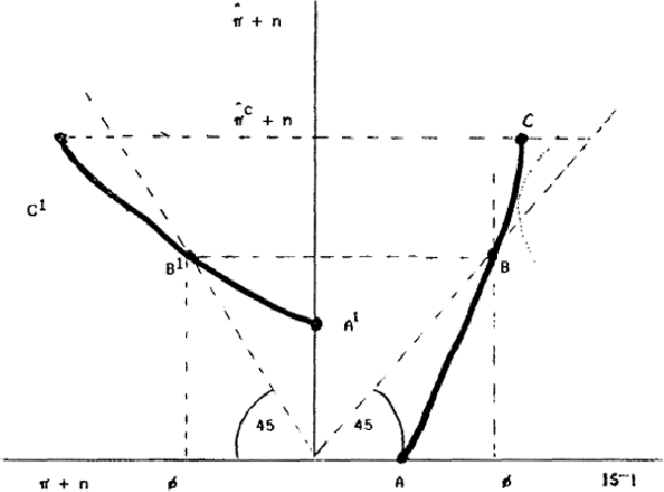
A negative debt gap will be associated with a positive inflation gap if the government is overly cautious. This causes output to start rising from its steady state. To show this, the sign of the eigenvalue, , has to be established. As before:

where A is the transition matrix in (28). Considering only the third column in [S⁺I−A] gives

Evidently, this is negative if θ>ρ. So from (30), the fiscal-induced negative debt gap will be associated with a positive inflation gap, and from (3), this will induce output to rise. The intuition behind this is that fiscally cautious governments are expected to rein in endogenous fiscal instruments in the future as debt accumulates. Hence future nominal demand is expected to fall, and with it inflation. Thus for t>0. Inflation must then overshoot its steady state value for this to be true. The converse occurs for governments that are not overly cautious and who set θ so that ρ−n/(1−α)<θ<ρ.

If the eigenvalues have no imaginary roots, cycles about the steady state cannot be experienced. In that case, it is manifestly clear that fiscally cautious governments will be able to create net output gains. The positive effects of the inflation gap will eventually be counteracted by the increasing output gap effect (via ϕ) on real wages. As in the previous section, the output gap will have an ambiguous influence on the inflation gap, via . Previously the relationship simply depended on (see (26)). Now using the second column of A

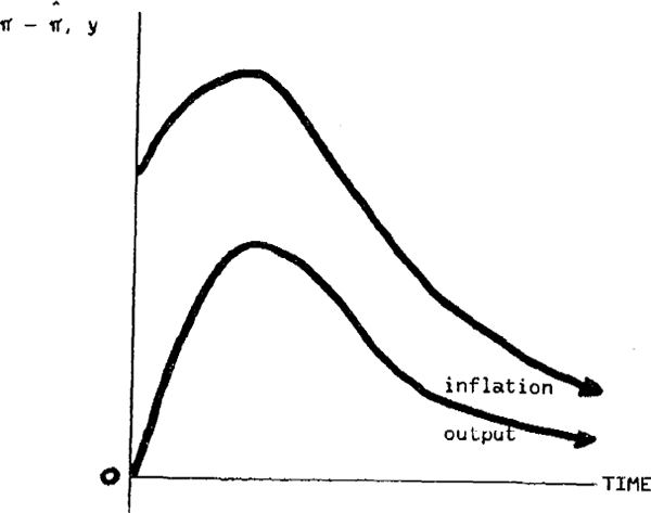
As mentioned with reference to (29), is expected to be negative. Hence, for a cautious government (θ>ρ), the likelihood of is definitely greater than in Section 3. If for a cautious government, then the initial positive inflation gap induced by the debt gap will initially be stimulated as the output gap becomes positive. When the output gap begins to fall later on, the inflation gap will follow suit. Hence stagflation (or its converse) would not be observed. This possible outcome is depicted in Figure 2a. 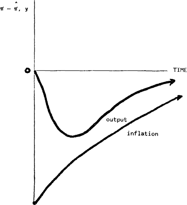If for a fiscally uncautious government, then the negative output gap would raise the negative inflation gap and so inflation would be observed to be rising throughout the adjustment period. in the initial phase, declining output and rising inflation – stagflation – would be observed. This outcome is shown in Figure 2b.

The net output or gain between two steady states (0 and 1) can be easily obtained regardless of whether the dynamics are characterised by cycles. We need to find . To proceed, (28) can be manipulated to eliminate and , and to end up with an equation for y as a linear function of , and . Integrating that over time, and noting that and we get

From the steady state equations, (12) and (13), a proportional increase in D_o, by say δ, leads to a linearised increase in and of the form

Inserting (34) in (33) gives

Evidently, this is positive for a fiscally cautious government (θ−ρ>0). For uncautious governments, a net loss is more likely as the share of money in deficit finance (α) decreases. If η or α are 0, fiscal policy is seen to be neutral. Non-neutrality can be achieved if money financing depends on fiscal policy and if real wages are forward looking.

These results are true only up to a point. As in the simpler model, the critical factor is that the exogenous fiscal deficit is sustainable. Fiscal pump-priming would cause the system to explode if the underlying inflation rate pierced its critical level as defined in (9).

Consider now a supply shock such as an oil price increase if energy were specified as a factor of production. Steady state output falls, but current output falls further because real wages will, initially, be too high. If taxes were independent of output, t=0, then would be unaffected. Otherwise must rise after the supply shock because equilibrium income taxes will have fallen. Hence negative output and debt gaps will be immediately created. The effect on the inflation gap is again ambiguous because cannot be signed. The only question that can be addressed is whether fiscal expansion can speed up the return of output to steady state. In the simple model without debt, the answer was in the affirmative and this was due to the change in . Fiscal expansion now worsens the debt gap, and this improves the inflation gap for a fiscally cautious government (given positive S⁺). This direct effect speeds up output adjustment. Further will increase in absolute size since the numerator in (31) is greater and the denominator will be smaller. The smaller denominator, as in the previous section, occurs because the stable eigenvalue decreases in size. Also will decrease (eventually turning negative) thereby further magnifying the output correction effect.

A fiscally cautious government can use expansionary fiscal policy to raise the speed of adjustment of output after a supply shock, provided the deficit is sustainable and monetary policy is not exogenous. For an uncautious government, the effectiveness is reduced.