
Statement on Monetary Policy – November 2026Box A: How Does an Increase in Longer-term Real Yields Affect Financial Conditions?
Longer-term real government yields have risen sharply across advanced economies in recent months. Whether this tightens financial conditions depends on why yields have risen. If yields have risen because markets expect stronger growth, the prospect of higher earnings and returns on investment can more than offset higher discount rates, thereby supporting asset prices and investment. If they have risen because markets expect more restrictive monetary policy or require a higher term premium, there is no such support and financial conditions are likely to have tightened. The recent rise in yields appears to reflect a mix of factors. In Australia, long-term yields have less direct influence on borrowing costs than in the United States because most borrowing here is at variable rates. However, this does not necessarily mean weak transmission overall: increases in foreign yields can still affect domestic financial conditions through asset prices and the exchange rate. This Box examines the drivers of longer-term real yields, places the recent increase in historical context, and considers how higher yields affect financial conditions in Australia.
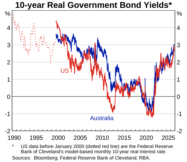
Longer-term real government yields have risen by as much as 85 basis points over 2026, reaching their highest levels since the early 2000s (Graph A.1). Most of this increase reflects higher real yields rather than changes in longer-term inflation expectations, which have remained broadly stable. The current increase is part of a broader and more sustained rise in longer-term yields since 2021 (see Box B: Developments in the Neutral Rate of Interest). Higher real yields do not necessarily imply tighter financial conditions. Their effect on financial conditions depends on what is driving the increase and how changes in long-term rates are transmitted through the economy.
What drives longer-term real yields?
Longer-term real yields reflect the expected path of future short-term real rates and a so-called ‘term premium’. Increases in real yields can be grouped into three broad drivers, with the first two working through expected policy rates:
- stronger expected growth: markets may expect stronger economic growth, which can raise expected real policy rates because the neutral rate is thought to have risen (e.g. because of higher productivity growth)
- other policy repricing: markets could expect policy rates to stay higher for longer for reasons other than stronger growth, such as when inflationary pressures lead markets to expect policy to remain restrictive (i.e. above the neutral rate) for a time, such as during persistent adverse supply shocks
- higher term premium: investors may demand greater compensation to hold longer-term bonds, above what they would demand to hold a series of equivalent shorter-term instruments, while expectations for growth and policy rates are little changed.
These drivers can have different implications for financial conditions. When higher yields reflect stronger expected growth, higher expected earnings and returns on investment can more than offset higher discount rates, thereby supporting asset prices. By contrast, when yields rise because of expectations of more restrictive monetary policy or a higher term premium, there is no comparable offset and financial conditions are more likely to tighten. In practice, yield movements can reflect a combination of these drivers.
Putting the recent increase in historical context.
The increase in real yields this year is notable, but not unprecedented. It is comparable in size with several previous episodes, including the dot-com boom, the pre-global financial crisis (GFC) expansion and the 2023 term premium sell-off (Graph A.2). The drivers of these episodes differed, however. Table A.1 classifies past episodes by our assessment of their predominant driver, based on contemporaneous market developments and revisions to consensus forecasts of activity, inflation and policy rates. Several episodes reflected more than one driver.
| Episode | Period | Description |
|---|---|---|
| Growth expectations | ||
| Dot-com boom | Oct 1998– Jan 2000 |
Optimism about technology and productivity supported a sharp rise in equity prices. Long-term growth forecasts rose substantially, while long-term inflation forecasts were broadly stable. |
| Pre-GFC expansion | Feb 2005– Jun 2007 |
Solid global growth, rising equity and housing prices and rapid credit growth pointed to optimism about future activity and returns. |
| Synchronised growth | Jul 2016– Nov 2018 |
A broad-based global upswing in economic activity, along with higher equity prices and compressed risk spreads. |
| Other policy repricing | ||
| ’94 Fed repricing | Oct 1993– Nov 1994 |
Stronger activity and concerns about prospective inflation, together with limited advance communication, left markets unprepared for the pace of monetary tightening, producing a sharp bond-market adjustment. |
| Post-pandemic reopening and Russian invasion of Ukraine | Nov 2021– Nov 2022 |
Reopening of economies, supply disruptions and the energy shock led markets to expect rapid monetary tightening; bond yields increased, equity prices declined, and growth forecasts were revised lower. |
| Term premium | ||
| Taper tantrum | Apr–Sep 2013 | The prospect of reduced asset purchases by the US Federal Reserve triggered a sharp bond sell-off and retrenchment from emerging-market assets. |
| Term premium sell-off | Apr–Oct 2023 | Increased government bond supply raised term premia and risky asset prices weakened as yields rose. |
| Mixed | ||
| Current episode | Feb 2026– | Stronger US earnings expectations, AI-related equity gains and modestly higher long-term growth forecasts point to a growth component. Increased bond issuance and quantitative tightening point to higher term premia, while expected policy rates have also risen. |
|
Source: RBA. |
||
The dot-com boom provides the clearest example of higher yields accompanying stronger expected longer-term growth. The pre-GFC and 2016–2018 synchronised growth periods were also associated with strong asset prices and economic activity, but forecasts at the time suggest that stronger growth was expected to be cyclical rather than structural. By contrast, the taper tantrum and 2023 term premium sell-off were associated with weaker asset prices and little change in long-term growth expectations, consistent with a larger role for term premia.
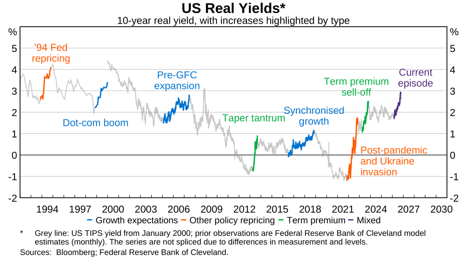
Historical experience also provides a useful reminder that the expectations underpinning market pricing are not always realised. In some cases, periods of strong optimism about future growth have given way to sharp falls in risk asset prices, notably following the dot-com boom and the expansion preceding the GFC. In others, interest rate markets may be slow to recognise lasting improvement in growth prospects.
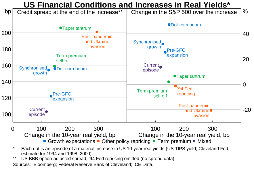
The current episode appears to reflect a combination of these drivers. In the United States, higher growth expectations appear to have contributed: rising yields have coincided with stronger earnings expectations and higher equity prices, particularly in AI-sensitive sectors, while credit spreads have remained near historical lows (Graph A.3). Expectations of a higher path for policy rates have also contributed. Increased debt issuance and ongoing quantitative tightening, alongside an investor base that is becoming more sensitive to expected returns, also appear to be placing upward pressure on term premia.
In Australia, however, the rise in yields has not been accompanied by a comparable improvement in growth expectations priced into financial assets. That is consistent with the much smaller AI-related sector here, and the less pronounced reassessment of the broader domestic economic outlook. Instead, the rise in Australian yields appears to reflect expectations of a higher path for the cash rate and spillovers from global yields (see Chapter 1: Financial Conditions and Box B: Developments in the Neutral Rate of Interest). As a small open economy, Australia is affected by global movements in longer-term yields, including in neutral rates and term premia, even when domestic fundamentals have changed little.
How do longer-term real yields affect financial conditions in Australia?
An increase in longer-term real yields can be transmitted into broader financial conditions through borrowing costs, asset prices, investment and the exchange rate. The overall effect on financial conditions depends on why yields have risen, with the three drivers discussed above having different implications for Australia.
When higher global yields reflect stronger expected growth, the implications for Australian financial conditions are ambiguous. If stronger growth is also expected for Australia, higher expected earnings and returns on investment may offset the effects of higher discount rates. But if the improvement in growth expectations is concentrated abroad, such as from AI-related investments, Australia may import some of the rise in long-term yields without receiving the same benefit of higher expected growth. In that case, the increase in global yields could tighten Australian financial conditions. A persistent productivity or growth differential (in favour of the United States for example) would also be expected to put downward pressure on the real exchange rate, which would provide some offset to the tightening in domestic financial conditions. Similarly, stronger overseas activity could provide some offset by lifting domestic incomes (through trade and commodity-price channels).
When higher yields reflect expectations of more restrictive monetary policy, financial conditions are more likely to tighten. Expected borrowing costs rise, while higher discount rates weigh on asset prices and investment. If Australian policy rates are expected to rise relative to those abroad, a higher exchange rate could tighten domestic conditions further.
When higher yields reflect a higher term premium, the direct effect on broader financial conditions depends partly on the economy’s exposure to longer-term rates. Differences in financing structures can therefore mean that the same rise in longer-term yields is transmitted differently across economies.
Australian household borrowing is concentrated in variable-rate mortgages, making borrowing costs less directly sensitive to term premia than in the United States (Table A.2). Thirty-year fixed-rate mortgages are common in the United States, which makes new borrowing rates sensitive to term premia but also means that changes in term premia can take a long time to affect average outstanding rates on mortgages. The differences are less clear-cut for business financing. Higher discount rates may have a larger direct effect on aggregate US equity indices because they are more heavily weighted towards technology companies, whose valuations depend heavily on earnings many years ahead.
| Australia | United States | United Kingdom | |
|---|---|---|---|
| Household borrowing | |||
| Effective period before mortgage rates reprice(a) | <1 month | 8.5 years (mostly 30-year fixed term) | 3 years (mostly fixed terms of 2–5 years) |
| Business borrowing(b) | |||
| Bank loan structure | 89 per cent variable-rate | Mostly variable-rate for larger businesses; mostly fixed-rate for small businesses | Mostly variable-rate |
| Bond tenor(c) | 6.0 years | 8.4 years | 8.3 years(d) |
| Bond/loan share | 19 per cent bonds | 39 per cent bonds | 24 per cent bonds |
| Government borrowing | |||
| Funding tenor(e) | 6.5 years | 5.9 years | 13.4 years |
|
(a) Effective period for which rates on outstanding mortgages are fixed. For
Australia and the United Kingdom, this is calculated as a weighted (by amount
outstanding) average of the fixed-rate period, with variable-rate mortgages treated as
able to reprice immediately; the Australian figure uses the residual term of the
fixed-rate period, while the UK figure uses original maturity due to data limitations.
The US estimate uses average duration of agency mortgage-backed securities. Sources: AOFM; APRA; Bank of England; Bloomberg; Federal Reserve; LSEG; Office for National Statistics; RBA; UK Debt Management Office; US Congress Joint Economic Committee. |
|||
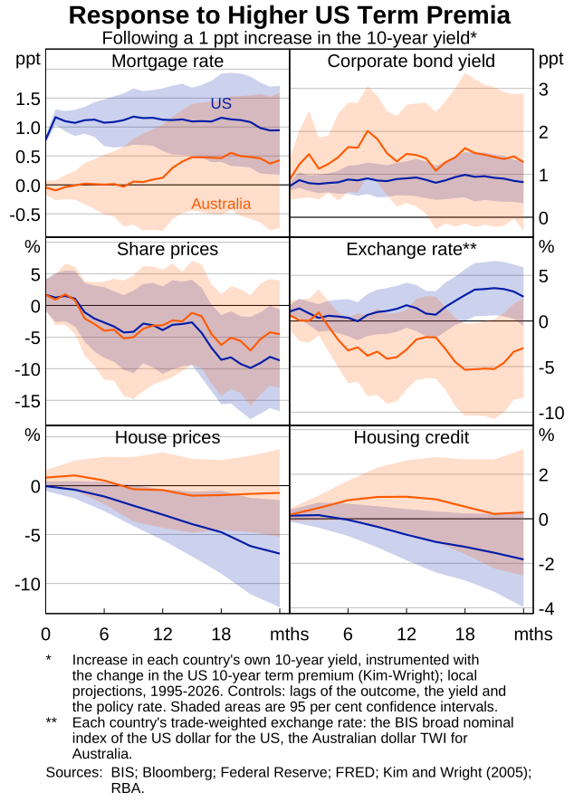
While differences in financial structures affect the direct transmission of higher yields to the economy, the overall effect on financial conditions also depends on broader responses in asset prices and other financial variables. Model-based estimates, using data from 1995 onwards, suggest that US term-premia-driven increases in longer-term yields have, on average, been associated with higher borrowing costs and lower equity and housing prices in both Australia and the United States (Graph A.4).1
As expected, these estimates show a larger impact on mortgage rates and housing prices in the United States than in Australia. By contrast, equity prices fall by at least as much in Australia as in the United States, illustrating that weaker direct pass-through to borrowing rates does not necessarily imply weaker transmission overall. Even so, the associated wealth effects from equity market holdings may be weaker in Australia than in the United States because a substantial share of Australian households’ equity wealth is held indirectly through superannuation, which is less readily accessible for consumption.2 The Australian dollar also tends to depreciate in such situations, partly offsetting the tightening in domestic financial conditions; this is consistent with a US term-premium shock raising US yields more than Australian yields.
Endnotes
1 The responses in Graph A.4 are estimated using local projections (Jordà O (2005), ‘Estimation and Inference of Impulse Responses by Local Projections’, American Economic Review, 95(1), pp 161–182), with the change in the US 10-year term premium (Kim D and J Wright (2005), ‘An Arbitrage-Free Three-Factor Term Structure Model and the Recent Behavior of Long-Term Yields and Distant-Horizon Forward Rates’, FEDS No 2005-33) used as an instrument for each market’s 10-year government bond yield. Because US term premium movements can reflect a range of underlying shocks, the estimates capture average historical associations rather than the effects of a specific structural shock. In addition, the term premium estimates we use are model-based decompositions that cannot always distinguish perfectly between increases in yields stemming from the term premium and those from other drivers such as growth expectations. For a small open economy like Australia, the instrumental variable approach nonetheless helps to separate movements in yields from developments affecting both yields and financial conditions (this interpretation is less straightforward for the United States). This means that some of the results in Graph A.4 – for instance, the slight increase in mortgage rates and housing credit – may reflect in part higher expected global growth instead of a ‘pure’ increase in the US term premium. The confidence intervals around these estimates are wide, particularly for Australia.
2 Equity ownership is more concentrated among wealthy households in the United States, which may reduce the aggregate consumption response because those households tend to have lower marginal propensities to consume out of stock market wealth. However, their large quantity of equity holdings means that they can still account for a substantial share of the aggregate consumption response to equity price movements (Mitra I and D Rapach (2026), ‘Downside Risk to the Stock Market and Consumption’, Federal Reserve Bank of Atlanta Policy Hub Series No 6-2026).