RDP 2025-06: An AI-powered Tool for Central Bank Business Liaisons: Quantitative Indicators and On-demand Insights from Firms Appendix A: Stratified Sampling to Assess Accuracy
August 2025
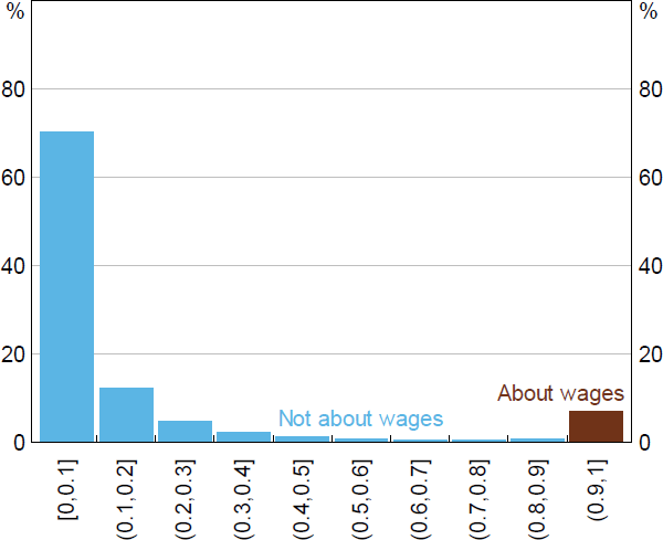
Most paragraphs in the liaison corpus are not about wages (or labour costs). Figure A1 shows the distribution of the LM's predicted probabilities for the wages topic. If we set the threshold for the LM to 0.9, then it would only classify 7 per cent of paragraphs to be about wages. If we randomly sample 600 paragraphs from this population we are unlikely to pick up many of these paragraphs – that is, we would expect to have only 42 paragraphs to assess. This can make it difficult to validate the performance of our method using metrics that rely on observing more than a few cases of wages paragraphs.

Sources: Authors' calculations; RBA.
The solution is to up-sample paragraphs that are likely to be about wages. We use the LM's distribution of predicted probabilities for wages to guide how we sample the population. First, we stratify the population based on the deciles of the distribution. Then we randomly sample an equal number of times from each of the deciles (or stratum). This method is known as stratified sampling.
To account for the imbalanced sampling of each stratum, we calculate an importance weight based on the sample's representativeness of the entire population. For example, a paragraph sampled from the [0,0.1] stratum (which contains about 70 per cent of paragraphs) would be 10 times more representative compared to a paragraph sampled from the (0.9,1] stratum (which is only 7 per cent of paragraphs). This is known as importance sampling and is often used to reduce the variance when estimating expected values of distributions. The importance sampling weighting formula for each of our stratums is given by:
where Ni is the number of instances in decile i in the (estimated) true population, and N is the total number of instances in the true population. The weighted F1 score is the sum of the F1 scores for each decile, weighted by their respective weights:
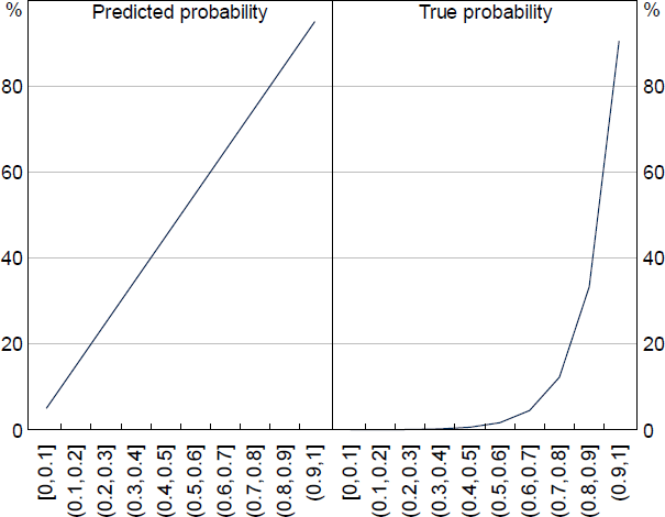
We can simulate a classification task on an imbalanced distribution to test if up-sampling helps improve the assessment of model performance. For the simulation, we have a population of 400,000 observations split into 10 stratums based on the distribution in Figure A1. Observations sampled from each stratum get assigned a predicted and true label based on the rates of predicted and true probabilities shown in Figure A2. The predicted probability is based on the LM's output, while the true probability is an estimation of the true positive rate based on spot checks of the real liaison data. For example, predictions below 0.6 in the real data are very rarely about wages, while most paragraphs observed discussing wages have a score above 0.9.

Sources: Authors' calculations; RBA.
In this simulation exercise, as a baseline, we randomly sample 600 observations from the whole population and calculate our performance metrics. Then we apply stratified sampling by taking 60 random observations from all 10 stratums. This ensures we up-sample observations more likely to be true. We account for the up-sampling by including the importance weighting of each stratum when calculating the performance metrics. We repeat this 1,000 times to calculate the mean and variance of each performance metric using both sampling methods.
We find that a sample of 600 observations on average gives a sufficiently accurate estimation of the true performance metrics for both methods. However, the variance of the metrics for the stratified sampling is lower than random sampling, especially for recall (almost three times smaller; see Table A1). This demonstrates that our stratified sampling method is more accurate given the large class imbalance in our data. This same method is used to up-sample wages paragraphs when validating our liaison wages measures.
| Metric | Full sample | Random sampling | Stratified sampling | |||
|---|---|---|---|---|---|---|
| Mean | Variance | Mean | Variance | |||
| Recall | 0.950 | 0.952 | 0.034 | 0.951 | 0.014 | |
| Precision | 0.908 | 0.907 | 0.045 | 0.909 | 0.036 | |
| F1 | 0.928 | 0.928 | 0.030 | 0.929 | 0.021 | |