RDP 2025-06: An AI-powered Tool for Central Bank Business Liaisons: Quantitative Indicators and On-demand Insights from Firms 5. An Empirical Application: Nowcasting Wages Growth
August 2025
5.1 Methodology
The capabilities introduced in the previous section have enabled staff to synthesise and transmit business intelligence collected through the RBA's extensive liaison program more efficiently and systematically. Among other things, use of these new capabilities over the recent period has supported the ongoing use of judgement in informing the RBA's assessment of current economic conditions – including the use of judgement informed by liaison intelligence to test and adjust forecasts derived from statistical models.
In this section, we demonstrate the potential of directly incorporating new liaison-based textual indicators into model-based nowcasts using machine learning methods. We apply this to nowcasting quarterly growth in the WPI for the private sector. Here, ‘nowcasting’ refers to estimating wages growth for the current quarter. A WPI nowcast can be an important policy input, as official statistics for the quarter are released with a 7-to-8-week lag.
We take three machine learning models that incorporate all relevant text-based information from liaison and compare each of them to a baseline Phillips curve model that is among the suite of best-performing models that have been used to nowcast wages growth at the RBA. We also benchmark against the RBA's expert judgement-based adjustment to the model-based nowcast for growth in the WPI for the private sector.
We set up the exercise to be as realistic as possible.[25] In practice, the model-based nowcast for quarterly growth in the private sector WPI, WPIt, is produced by staff around the end of the reference quarter (Figure 12). This nowcast uses the recently released figure for wages growth in the previous quarter. About one month after the model-based nowcast is produced, senior staff finalise their judgement-based nowcast for wages growth, which takes the model-based estimate and adjusts it using liaison intelligence and other timely information. This judgement-based nowcast is published in the RBA's flagship monetary policy publication, the Statement on Monetary Policy.
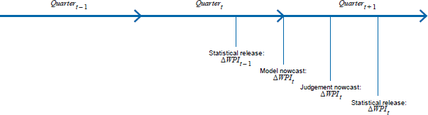
For example, imagine we were nowcasting for the June quarter 2020. Official data for the March quarter 2020, WPIMQ2020, were released on 13 May and a model-based nowcast for the June quarter was produced shortly thereafter. One week before the publication of the Statement on Monetary Policy on 7 August 2020, senior staff finalised their judgement-based nowcast for wages growth for the June quarter, with the official measure, WPIJQ2020, then published on 12 August 2020. This gives us a model- and judgement-based nowcasting error to analyse.
In producing the model-based nowcast, staff have available to them the following baseline Phillips curve model, which is estimated via ordinary least squares (OLS) regression by minimising the sum of the squared errors:
Here UnempGap is the gap between the unemployment rate and the RBA's latest assessment of the non-accelerating inflation rate of unemployment (NAIRU); UnutilGap is the gap between the underutilisation rate and the non-accelerating inflation rate of labour underutilisation (NAIRLU); and InfExp is a measure of inflation expectations from financial markets and surveys. At the time of nowcasting, these variables are only available to a nowcaster for the previous quarter (full definitions of all variables can be found in Table C1). To estimate the gap terms, staff use a model average estimate for the NAIRU and NAIRLU; importantly, these estimates are derived from one-sided Kalman filters that only use past information.
To this, we add 22 additional text-based variables Xi,t and their one-period lags Xi,t−1, all extracted from the liaison corpus to create an augmented baseline model. These additional variables include topic exposure and topic-specific tone measures for wages and labour (both LM- and dictionary-based); interaction terms between topic exposure and topic-specific tone; as well as our numerical extractions for firms' self-reported wages growth. We interact topic exposure with topic-specific tone to allow the marginal effect of tone to vary according to how much firms are talking about a specific topic – when a topic is font-of-mind, we would expect the marginal impact of a change in tone to be larger. When focusing on numerical extractions, we include the mean across all firms in each period.
Because there are over 44 covariates to estimate, we employ machine-learning-based shrinkage methods to avoid serious overfitting and associated poor nowcasting performance. The first of these is ridge regression:
Ridge regression shrinks the regression coefficients by imposing a penalty on their size. The ridge coefficients minimise a penalised sum of the squared errors, with controlling the amount of shrinkage. Shrinkage via ridge regression is potentially well suited to our nowcasting exercise because we have several variables (or features) that measure the same underlying concept (e.g. topic exposure) and that are highly correlated. Ridge regression shrinks coefficients that are similarly sized toward zero and those of strongly correlated variables toward each other. The penalty parameter, is adaptively chosen via cross-validation for every nowcast (discussed below).
The second method is the least absolute shrinkage and selection operator (lasso), which is a shrinkage method like ridge, but the penalty is based on the absolute size of the coefficients rather than their square:
Because of the nature of the penalty, making sufficiently large means lasso performs variable selection by pushing a subset of the coefficients to exactly zero during optimisation, effectively performing model selection.[26] As with the penalty parameter in ridge regression, it is adaptively chosen for every nowcast using cross-validation.
The lasso is a sparse modelling technique that selects a small set of explanatory variables with the highest predictive power, out of a much larger pool of regressors. On the other hand, the ridge regression is a dense-modelling technique, recognising that all possible explanatory variables might be important for prediction, although their individual impact might be small. An important contribution of this paper is to demonstrate that, when nowcasting wages growth in our exercise, the signal from text-based indicators extracted from business intelligence information is sparse rather than dense.
Finally, our third shrinkage method, elastic net, mixes the strengths of both the ridge and lasso methods, by performing variable selection like the lasso and shrinking together the coefficients of correlated features like ridge. The elastic net constraint is given below:
where determines the mix of the penalties and is chosen via cross-validation.
At the outset of our nowcasting exercise, we make a variety of decisions regarding our implementation strategy that are used across all three models, including defining the testing period, opting for either a rolling window or a recursively updating window and selecting a cross-validation procedure. These decisions are detailed in Table 3.
| Decision | Description | Choice |
|---|---|---|
| Pure training period | Initial period used to estimate model coefficients. | March 2006 to December 2014; 36 observations |
| Nowcasting period | The period used to evaluate nowcasting accuracy. | March 2015 to September 2024; 39 nowcasts |
| Window type | Whether to use a rolling or recursively updating window for model estimation. | Recursively updated |
| Benchmark model | Model against which nowcasting performance is compared. | Autoregressive distributed lag Phillips curve model |
| Data transformation | Transformation applied to the data. | All variables standardised to have a mean of 0 and a standard deviation of 1 for every nowcast |
| Evaluation metrics | Metrics used to evaluate the forecast performance. | Root mean squared error (RMSE) |
| Hyperparameter range | The range of and values to search over when selecting an optimal model. | = [0,7] 101 steps = [0,1] 10 steps |
We produce nowcasts for each quarter over the period March 2015 to September 2024 (a total of 39 quarters). The data available to train the model for each nowcast expands as we move forward. The first out-of-sample (OOS) nowcast, for March 2015, is based on the 36 quarters of pure training data. The next nowcast, for June 2015 uses the 36 training data points in addition to March 2015 and so on (Figure 13, top panel).
To run our ridge, lasso and elastic net regressions we must choose optimal values for the regularisation strength () and the mixing parameter in the elastic net – the so-called hyperparameters. We do this via time series cross-validation (CV). For each of the 39 nowcasts, we remove the data point for the final quarter (that we ultimately wish to predict) and divide the remaining observations into 10 folds (Figure 13, bottom panel). These folds are used to optimally select values for and , where the model is trained on past observations and evaluated, using the RMSE as a metric, on the last observation within each fold. Within each fold, a grid search is used to iterate through all possible combinations of the hyperparameters. The combination of hyperparameters that result in the lowest average RMSE error across all folds is then selected.
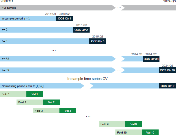
To illustrate this process, Figure 14 shows the selection of the optimal value of and (i.e. the regularisation strength) for the September 2024 nowcast. The optimal value for the ridge regression ( = 6.9) is not shown. The training data is the period from March 2015 to June 2024 and is split into the 10 CV folds. The x-axis shows a subset of the grid of values of that were tested, from 0 to 0.5, and the y-axis is the average of the RMSE values from predicting the final holdout sample across all 10 CV folds. For each model, we select the value of that minimises the average RMSE across all folds (optimal values are shown as dashed vertical lines for the lasso and elastic net models). In this case, the best performing model is lasso as the RMSE of the optimised lasso is slightly lower than the optimised elastic net model (and ridge, which is not shown).

Notes:
Dashed lines show optimal values of .
(a) The mixing weight for the elastic net regression is fixed at 0.56.
(b) For illustrative purposes, the optimal value for the ridge regression ( = 6.9) is not shown.
Sources: Authors' calculations; RBA.
5.2 Results
We find that nowcasting performance significantly improves with the use of shrinkage methods and the incorporation of our text-based indicators from liaison. In the case of wages growth, at least, this underscores the ongoing use of liaison to inform the RBA's assessment of current economic conditions – including by adjusting nowcasts derived from models using judgement informed by liaison intelligence. It also highlights the usefulness of our new text analytics and information retrieval tool, which both facilitates the on-demand construction of various text-based indicators and offers a way to identify which of these indicators are most useful for nowcasting.
In nowcasting wages growth, the lasso model incorporating all variables achieves significant improvements of almost 40 per cent relative to the baseline Phillips curve model estimated by OLS over the pre-COVID-19 sample (Table 4). Most of these gains come from simply applying shrinkage methods to the current baseline Phillips curve model. These shrinkage methods are useful in extracting a combined signal from the unemployment gap (UnempGap) and the underutilisation gap (UnutilGap). Incremental improvements are also made by incorporating the additional liaison-based indicators (plus their lags) using the lasso method. Notably, over the pre-COVID-19 sample, the best-performing nowcast from the lasso model that incorporates all variables outperforms the expert judgement-based nowcast by 20 per cent.
Over the full sample, all shrinkage-based estimators incorporating all variables achieve significant improvements of 20 per cent relative to the baseline OLS model. Over the full sample, the incorporation of additional liaison-based information makes a larger contribution to nowcasting accuracy, improving upon the regularised baseline by 12 basis points compared to 3 basis points over the pre-COVID-19 sample. This highlights the usefulness of incorporating timely liaison-based information during periods when the economic landscape is rapidly evolving, as was the case during and after the pandemic. This notwithstanding, the shrinkage-based nowcasts that incorporate all variables underperform the expert judgement-based nowcast. This is because the judgement-based nowcast significantly outperformed over the first half of 2020 during the onset of the pandemic – abstracting from this period, the shrinkage-based nowcasts are on par with the performance of the judgement-based nowcast.
| Pre-COVID-19 nowcasting sample (March 2015–December 2019) |
Full nowcasting sample (March 2015–September 2024) |
||||
|---|---|---|---|---|---|
| RMSE | Ratio to baseline OLS | RMSE | Ratio to baseline OLS | ||
| Baseline | |||||
| OLS | 0.089 | 1.00 | 0.192 | 1.00 | |
| Regularised baseline | |||||
| Ridge | 0.058 | 0.65*** | 0.176 | 0.91 | |
| Lasso | 0.061 | 0.69*** | 0.182 | 0.95 | |
| Elastic net | 0.059 | 0.66*** | 0.177 | 0.92 | |
| All variables(a) | |||||
| OLS | 3.093 | 34.67 | 2.236 | 11.62 | |
| Ridge | 0.064 | 0.71 | 0.152 | 0.79** | |
| Lasso | 0.055 | 0.62** | 0.153 | 0.80** | |
| Elastic net | 0.061 | 0.68* | 0.154 | 0.80** | |
| Judgement-based | |||||
| RBA published(b) | 0.069 | 0.78* | 0.133 | 0.69** | |
|
Notes: ***, ** and * denote statistical significance of nowcasting performance differences at the
1, 5 and 10 per cent levels, respectively from a Diebold and Mariano test. Shading signifies the
best performing model over each sample range. Sources: ABS; Authors' calculations; RBA. |
|||||
The results from an OLS regression including the full set of liaison indicators significantly overfits the data, resulting in poor nowcasting performance relative to the baseline model. This highlights the importance of using methods to shrink or reduce the dimensionality of the feature space.
Over the pre-COVID-19 sample, the lasso regression applied to all variables outperforms the ridge and elastic net methods. Over the full sample, all shrinkage-based methods perform similarly. For the ridge regression to perform well over the full sample, a large degree of shrinkage is imposed over the post-COVID-19 period. Taken together, these results suggest that sparse models may produce better predictive performance in this context.
To get a sense of the degree of sparsity, for each predictor we can examine how many times it is selected in the lasso model. That is, out of the 39 nowcasts, how many times is each predictor selected in the optimal model? The results, shown in Appendix D (see Figure D1), show that only seven predictors are included in the optimal model in more than half of the nowcasts, with around 40 per cent of the predictors never selected for inclusion in the optimal model. The finding of a sparse signal is important. Previous work by Giannone, Lenza, and Primiceri (2021) across a variety of applications in macroeconomics suggests that predictive models often benefit from including a wide set of predictors rather than relying on a sparse subset. Our results indicate this is not always the case when incorporating text-based indicators from corporate intelligence into predictive models.
Given these results, we can now examine the identity of the relevant predictors. The underutilisation gap and inflation expectations variables, which are features of the baseline Phillips curve model, are frequently selected in the all-variables lasso model (Figure 15). This is unsurprising as their inclusion is based on strong theoretical relationships. The lagged ordinal staff score for expected wages growth is selected in all periods. Several other traditional liaison-based measures from staff scores are also selected frequently over the pre-COVID-19 period, including for firms' expected prices and employment intentions. Turning to the new text-based indicators, we see that firms' self-reported wages growth estimates – hand collected and extracted using LMs – are selected in all nowcasting periods. The frequency with which firms talk about the labour market as measured by the LM-based topic exposure ( or its lag) also adds incremental nowcasting value in almost all periods. The liaison-based uncertainty index is also useful. Finally, in the pre-COVID-19 period, interactions between topic exposure for wages and the associated tone of the discussion is selected in almost every period, indicating that the marginal impact of tone depends on how often the associated topic is mentioned.
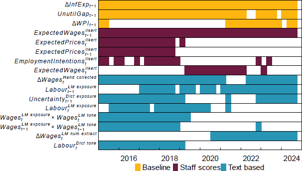
Note: Only showing variables that were selected in at least 10 or more nowcasts.
Sources: Authors' calculations; RBA.
Summing up, integrating timely text-based liaison information into wages nowcasts makes them more responsive to new on-the-ground insights from firms and improves nowcasting performance. Indeed, access to more timely information and increasing the responsiveness of nowcasts to incoming information were key recommendations from the RBA's review of its forecasting performance at the time (see RBA (2022b)).
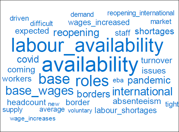
To see why these lessons are important, a specific error analysis of the nowcasts is useful. Over the year to September 2022 quarterly nowcast errors for wages growth from the baseline Phillips curve model were among the largest over our nowcasting period. In hindsight this was due to various supply-side factors that limited the available pool of skilled labour, which the baseline model does not capture very well. According to the baseline Phillips curve model, growth in wages over the year to September 2022 was estimated to be 2.7 per cent, compared to realised growth of 3.4 per cent, with the 70 basis point error due to a series of quarterly nowcasting errors underestimating growth in wages. While liaison information was considered as part of the nowcasting process at the time, the formal incorporation of timely liaison text-based indicators would have reduced the model error to around 20 basis points. To understand why we can drill down into the micro level of the liaison text over this period. Focusing on text snippets that mention the labour market (recalling that was a significant predictor during this period), we can identify words or n -grams used in the liaison summaries over the period that appeared at an unusually high frequency compared to other years.[27]
The results shown in Figure 16 point to a challenging labour market in 2022, characterised by staff shortages, wage pressures and the ongoing effects of the pandemic, with a significant emphasis on international factors. In practice, upward judgements informed by these liaison messages were increasingly incorporated into the nowcasts for wages over 2022, and the above results affirm that this was a sensible judgement to make. However, formally incorporating this information via our text-based indicators, had the tool and these indicators been available at the time, could potentially have provided a more accurate starting point from which to apply judgement if deemed necessary.
Sources: Authors' calculations; RBA.
Footnotes
There remains a small element of look-ahead bias in our nowcasting exercise. This is because a staff member producing the nowcast would not have had access to large pre-trained LMs over most of the sample period. Pre-trained LMs are necessary to construct several of our liaison-based textual indicators. This notwithstanding, the nowcasting improvements we report are qualitatively similar (albeit slightly weaker) if we only use our keyword-based indices (which are not subject to this look-ahead bias). Further, a nowcaster would have had access to human judgement based on the liaison corpus, which is available over the entire sample period. [25]
Lasso can be interpreted as placing a Laplace prior on the distribution of the coefficients, which peaks sharply around zero as opposed to ridge which can be interpreted as a Gaussian prior. [26]
To do this we calculate the class-based term frequency-inverse document frequency (c-TF-IDF). This is an expanded version of traditional TF-IDF, and is often used in topic models, such as BERTopic for class identification. In this case, our identified class is all snippets of text in 2022 that were classified into the ‘labour’ topic using the LM-based approach. From this we extract terms (including bigrams) which having the highest TF-IDF score. A high score indicates a term was used at an unusually high frequency in 2022, relative to other years. [27]