RDP 2020-01: Credit Spreads, Monetary Policy and the Price Puzzle Appendix D: Further Robustness Tests and Results
January 2020
- Download the Paper 460KB
D.1 SVAR Misspecification
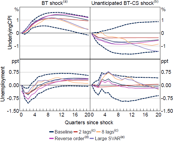
In addition to adding domestic and credit market spreads to the baseline SVAR, I find my results to be robust to other SVAR specifications (Figure D1). These are: (i) choosing shorter or longer lag orders for the VAR (2 or 8 lags); (ii) ordering the policy shock first; and (iii) augmenting the SVAR by the Bank's commodity price index (in logs), the nominal trade-weighted exchange rate index (nominal TWI, in logs), and the US federal funds rate (Jacobs and Rayner 2012). Ordering the policy shock first allows monetary policy to have immediate effects on all endogenous variables in the VAR and reflects that the obtained policy shock series should already be exogenous to the state of the economy to the extent that this is captured by the Bank's forecasts. The SVAR with the policy shock ordered first and the augmented SVAR suggest slightly larger price effects, while both the augmented SVAR and a SVAR with longer lags suggest larger peak unemployment effects.

Notes:
See notes for Figures 7 and 9
(a) Original, anticipated policy shock used by Bishop and Tulip (2017)
(b) New, preferred unanticipated policy shock
(c) Baseline SVAR with 2 or 8 lags
(d) Cumulative policy shock ordered first
(e) Baseline SVAR augmented by RBA index of commodity prices, US federal funds rate and the Australian nominal TWI; nominal TWI ordered last
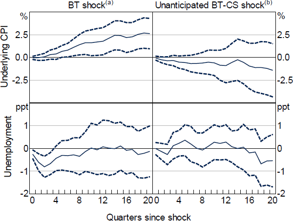
I further find my results to be largely robust when estimating the effects of a cash rate change using the univariate LP framework introduced by Jordà (2005).[28] Here, impulse responses are obtained by estimating the effects of monetary policy directly as:
where is the long difference in the variable of interest from the end of quarter t to t + h, that is is the quarterly difference in yt and Xt is a vector of additional macroeconomic controls.[29] In contrast to the identifying assumption of the SVAR, the LP framework allows for an immediate effect of a monetary policy shock on the dependent variable.[30] The parameter provides the estimate for the change in the variable of interest between end of quarter t and t + h attributed to the monetary policy shock occurring during quarter t + 1.
Overall, the results from the regressions are very similar to the SVAR results (Figure D2). In particular, I find no evidence of a price puzzle when using the new preferred, unanticipated BT-CS shock. However, the unemployment response is smaller and appears to be negative in the long run.

Notes:
Dashed lines show 90% heteroskedasticity and autocorrelation robust confidence intervals
(a) Original, anticipated policy sock used by Bishop and Tulip (2017)
(b) New, preferred unanticipated policy shock
D.2 Different Cash Rate Reaction Function
To allow comparison between the estimates, I followed the Bishop and Tulip (2017) specification for the RR regression which includes the lagged level of the cash rate and the nowcast of the unemployment rate. One possibility is that the inclusion of credit spreads just captures other variables to which the Bank responds when setting the cash rate and that the baseline Taylor rule is hence misspecified. Accordingly, I find that two changes to this benchmark specification increase the fit of the model considerably even before adding any money and credit market spreads. Specifically, I replace the lagged level of the cash rate with the previous change in the cash rate and the nowcast of the unemployment rate with the two-quarter-ahead forecast. Both coefficients are statistically significant and increase the model fit from around 25 to 40 per cent (Table D1, regression BT). Furthermore, I find a small but significant response of the cash rate to variables capturing international conditions, in particular commodity price inflation , albeit with an unexpected, negative sign) and the nominal trade-weighted exchange rate . This may suggest that the cash rate in part responds to the global (financial) cycle.
| Variable | BT | BT-CS1 | BT-CS2 | BT-CS3 | BT-CS | BT-Int | BT-CS-Int |
|---|---|---|---|---|---|---|---|
| Constant | −0.18 | 0.06 | −0.01 | −0.05 | 0.27** | −0.16 | 0.22* |
| 0.35*** | 0.20** | 0.33*** | 0.31*** | 0.17* | 0.24** | 0.12 | |
| 0.07** | 0.03 | 0.08** | 0.08** | 0.04 | 0.07** | 0.03 | |
| 0.01 | −0.01 | 0.01 | 0.00 | −0.01 | 0.01 | −0.01 | |
| −0.32*** | −0.20** | −0.34*** | −0.25** | −0.19** | −0.36*** | −0.28*** | |
| 0.21*** | 0.20*** | 0.16** | 0.21*** | 0.15** | 0.23*** | 0.18*** | |
| 0.11*** | 0.08*** | 0.13*** | 0.11*** | 0.10*** | 0.09*** | 0.09*** | |
| −0.56*** | −0.52*** | −0.48*** | |||||
| −0.08*** | −0.08*** | −0.09*** | |||||
| −0.05 | −0.03 | 0.01 | |||||
| 0.01 | 0.02* | ||||||
| ntwit | 0.02*** | 0.01*** | |||||
| 0.00 | −0.00 | ||||||
| Observations | 100 | 100 | 100 | 100 | 100 | 100 | 100 |
| R 2 | 0.430 | 0.561 | 0.480 | 0.445 | 0.607 | 0.536 | 0.692 |
| Adjusted R 2 | 0.393 | 0.527*** | 0.440*** | 0.403 | 0.568*** | 0.490 | 0.650*** |
| Notes: Statistical significance of the difference in model fit (Adjusted R 2) to the benchmark (excluding credit spreads or international variables) is assessed using a likelihood ratio test; see Table 1 for further notes | |||||||
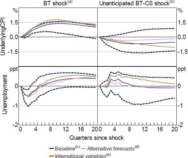
Nonetheless, credit market spreads still add significant explanatory value for cash rate changes to these alternative baseline specifications. Similarly, these changes to the BT regression have no material impact on the estimated impulse responses (Figure D3). The price puzzle disappears only when controlling for the response of the cash rate to credit market conditions and taking into account the anticipation of cash rate changes by financial market participants. When including international conditions to the alternative RR regressions, the effects of a cash rate change are slightly more contractionary for both inflation and the unemployment rate.

Notes:
Impulse responses to policy shocks obtained from alternative baseline Taylor rule regression (Table D1), see Figures 7 and 9 for further notes
(a) Original, anticipated policy shock used by Bishop and Tulip (2017)
(b) New, preferred unanticipated policy shock
(c) Original Taylor rule specification used by Bishop and Tulip (2017)
(d) Alternative Taylor rule specification (regression BT-CS of Table D1)
(e) Alternative Taylor rule specification including international conditions (regression BT-CS-Int of Table D1)
D.3 Further Results
Credit market conditions and inflation forecast errors across all horizons
| Predictor | Horizon (in quarters) | |||||||
|---|---|---|---|---|---|---|---|---|
| 1 | 2 | 6 | 8 | |||||
| Constant | −0.11 | −0.06 | −0.38* | −0.10 | −0.03 | 1.37* | 1.08* | 2.97** |
| −1.41*** | −1.44*** | −1.15*** | −1.24*** | 1.17*** | 0.88** | 1.75** | 1.48 | |
| 0.04 | 0.03 | 0.02 | 0.04 | −0.15 | 0.09 | −0.35 | −0.05 | |
| 0.06 | 0.07* | 0.10 | 0.10 | 0.31* | 0.31** | 0.45* | 0.39* | |
| 0.10 | −0.32* | −0.80* | −0.51 | |||||
| −0.03 | −0.10 | −0.43* | −0.63 | |||||
| Observations | 96 | 96 | 95 | 95 | 87 | 87 | 78 | 78 |
| R 2 | 0.784 | 0.786 | 0.391 | 0.417 | 0.375 | 0.370*** | 0.234 | 0.311** |
| F-statistic | 45.75*** | 35.05*** | 7.99*** | 6.74*** | 3.94*** | 5.12*** | 3.05*** | 3.41*** |
| Note: See Table 4 for notes | ||||||||
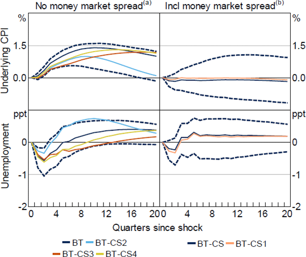
Estimated effects of monetary policy: the role of individual credit spreads measures

Notes:
Impulse responses from the benchmark recursive SVAR with one of the policy shocks from Table 1, see Figure 7 for further notes
(a) Bishop and Tulip ((2017), updated, BT) policy shock with confidence intervals, or BT shock accounting for cash rate response to domestic lending rate spread (BT-CS2), US corporate bond spread (BT-CS3) or US VIX (BT-CS4)
(b) BT shock accounting for cash rate response to all credit spread measures (BT-CS) with confidence intervals, or BT shock accounting for cash rate response to domestic money market spread (BT-CS1)
Footnotes
This framework allows estimating the effects of monetary policy without imposing the heavy parametric structure of the SVAR. Plagborg-Møller and Wolf (2019) show that this approach is conceptually identical to the SVAR approach and estimates the same impulse responses. However, and analogous to the choice between ‘direct’ and ‘iterated’ multi-horizon forecasting, VAR impulse responses (iterated) are more efficient if the chosen VAR accurately describes the data-generating process, whilst LP impulse responses (direct) are more robust to model misspecification. [28]
I include quarterly inflation, the quarterly growth rate of real GDP, and the change in the unemployment rate unless already included in the autoregressive term . I set P = Q = 4 and R = 1. Adding controls and lagged monetary policy shocks may provide more precisely estimated effects and soak up any residual autocorrelation in the shocks. [29]
I include all macroeconomic controls with a lag. Including simultaneous realisations of Xt may bias the coefficient of interest if the monetary policy shock affects these controls contemporaneously. As such, LP regressions including contemporaneous realisations of the controls impose the same timing assumptions as the standard, Cholesky-identified SVAR. Ramey (2016) finds that these timing assumptions are not innocuous. [30]