RDP 2018-02: Affine Endeavour: Estimating a Joint Model of the Nominal and Real Term Structures of Interest Rates in Australia 3. Data and Estimation
February 2018
- Download the Paper 1,673KB
3.1 Estimation
As discussed in JSZ, maximising the model likelihood conditional on the observed factors imposes the assumption that the factors are ‘priced correctly’ – essentially, that there are no (or limited) measurement errors or breaches of no arbitrage conditions – but has the benefit of exploiting the JSZ technique to significantly speed up estimation. This is likely to be a reasonably strong assumption in our case given the limited number of inflation-linked bonds trading at any one time.
For this reason we use a two-step estimation procedure. First, we maximise the model likelihood conditional on the observed factors.[9] In doing so we cannot separately estimate the P dynamics in this first estimation step, as the modelled counterparts of the surveys rely on both the P parameters and some other parameters used to price bonds, such as the inflation parameters. Instead, we jointly maximise the likelihood function of the observed factors, the observed yields and the surveys (all the while holding the pricing factors fixed as the principal components of the relevant yield data). We use VAR estimates of the P parameters as starting points for this optimisation. The model is more difficult to estimate than in the standard JSZ set-up without survey data, but it is still simpler to estimate than earlier approaches as the dependency between the P and Q parameters remains relatively weak under the JSZ normalisation.
In the second step we relax the assumption that the factors are priced correctly by casting the model in terms of a Kalman filter and re-optimising using the parameter estimates from the first step as starting values.[10] Relaxing the assumption that the factors are priced correctly has two benefits: it allows us to model estimates of real zero-coupon yields as being noisy and/or observed with error, which, as discussed above, is useful given the limited number of inflation-linked bonds trading at any one time; and it allows the survey data to affect the factors, as they should. The Kalman filter also gives us scope to drop real zero-coupon yields from the model if there are no inflation-indexed bonds with similar maturities outstanding. Such data points are likely to be particularly noisy and relatively more dependent on the interpolation method employed, and so dropping them should increase the robustness of our estimates.[11]
The allowance for noise means that Equations (4) and (7) become
where  and
and  . We also allow for errors/uncertainty in the survey responses. Instead of calibrating the variance of these errors, we allow them to be estimated alongside the other parameters. This approach is more common in the literature and allows the data to ‘speak for itself’. We assume that the errors are independent, homoskedastic and normally distributed, and allow the error variances to differ for each type of forecast data that we use.
3.2 Data and Observable Factors
For the first stage of the estimation we need a set of observable factors that are linear functions of the yields. Consistent with Abrahams et al (2016) we use the first K principal components from a panel of nominal interest rates. We also use the first L principal components from a panel of real yields that have been orthogonalised with respect to the nominal factors by regressing the real yields on the nominal factors using OLS; these factors will tend to capture divergences between the nominal and real yield data. Motivated by our findings with a purely nominal model, we use three factors extracted from the nominal yield data.[12] We considered using two or three factors extracted from the real yield data, and found that two factors were preferable based on parsimony and likelihood ratio tests.[13] Consistent with the vast majority of the literature, we impose that the P dynamics of the factors are stationary.[14]
Our nominal data consist of nominal zero-coupon yields estimated using the methodology in Finlay and Chambers (2009), with maturities of n = 6, 12, 18, 24, 36,…, 120 months. Our real data consist of real zero-coupon yields bootstrapped using linear interpolation.[15] For the initial stage of estimation we use maturities of n = 24, 36,…, 180 months.[16] Descriptive statistics are contained in Appendix D. For the second stage of estimation we only include real yield data if there is an inflation-indexed bond with a similar maturity outstanding. The sample period is July 1992 to December 2016, but we only show model estimates from 1993 onwards to abstract from issues related to the starting point of the Kalman filter.
We use two sets of surveys:
- Surveys on cash rate expectations obtained from the RBA survey of market economists and Bloomberg; and
- Surveys of inflation expectations from Consensus Economics. These included forecasts of year-average inflation a number of years into the future (available at a monthly frequency), forecasts of year-average inflation in the coming quarters (available at a quarterly frequency), and estimates of average inflation over a five-year period beginning in five years (‘five-year five-year forward’; available semiannually).
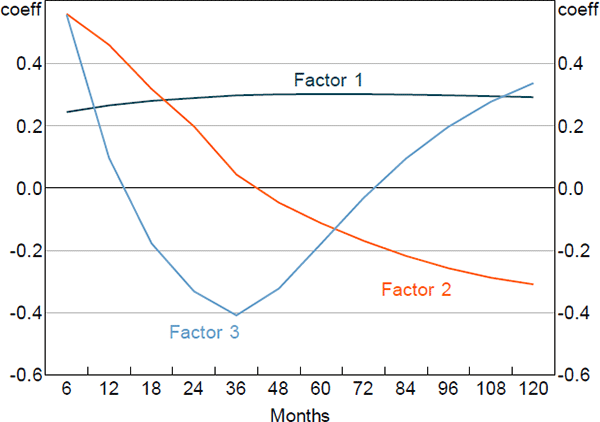
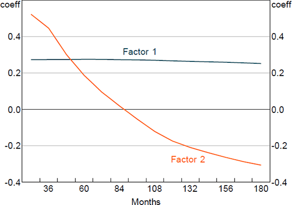
Figures 1 and 2 show the principal component loadings on the nominal and orthogonalised real yield data of various maturities. As is typically found in the literature, the nominal factors appear to reflect the level, slope and curvature of the nominal yield curve. Interpretation is more complicated for the factors extracted from the real data as they have been orthogonalised with respect to the nominal factors. Nonetheless, the loadings suggest that these factors are again related to level and slope.


Footnotes
Consistent with papers such as Adrian et al (2013), Abrahams et al (2016) and Malik and Meldrum (2016), we constrain the steady-state level of the pricing factors to be their sample averages. This helps to avoid small-sample biases. [9]
We initialise the Kalman filter factors using the level of the observed principal component factors. We also use a few different starting points for the parameters based on the first step of the estimation to help ensure we find a global, not local, maximum. [10]
The results are, in fact, reasonably robust to not dropping these yields. [11]
While a number of papers have argued that yields are not ‘spanned’ by the first three principal components of the yield curve (e.g. Cochrane and Piazzesi 2005; Joslin, Priebsch and Singleton 2014), Bauer and Hamilton (2017) show that standard tests lack power, and that properly accounting for this leads to less evidence that three factors are insufficient. [12]
One could also extract pricing factors from a joint panel of nominal and real yield data, although in practice both methods deliver factors that are essentially linear combinations of the other, and both sets of factors explain over 99.9 per cent of the variation in the nominal and real yield data. [13]
Malik and Meldrum (2016) find that models that instead impose a unit root tend to perform poorly. [14]
See Appendix C for further details. Another approach would have been to use the indexed bond prices directly as in Finlay and Wende (2012). However, this approach is not well suited to the JSZ normalisation. It would also require a nonlinear Kalman filter. Given that we want the model to be simple enough to be used on an ongoing basis, we eschewed this option. [15]
Liaison suggests that inflation-linked bonds provide the most reliable information on expectations between around three and ten years. Nevertheless, we use a wider range of yields because of the sparsity of traded bonds. [16]

