RDP 2018-02: Affine Endeavour: Estimating a Joint Model of the Nominal and Real Term Structures of Interest Rates in Australia Appendix B: The JSZ Normalisation
February 2018
- Download the Paper 1,673KB
To estimate the model we need to impose some parameter restrictions to ensure econometric identification. There are a number of different normalisations one can use; we use that from JSZ for the reasons outlined in the main text. The JSZ normalisation is formulated for standard nominal ATSMs rather than joint nominal–real models, and is not set up to incorporate survey data. As such, we need to adapt JSZ to deal with real yields and survey data, which we do now.
Focusing first on the result from JSZ regarding estimation with observable factors in which separation of P and Q parameters in estimation is achieved (‘Case P’ in JSZ), Proposition 1 of JSZ gives the key result that any standard ATSM with the representation
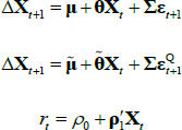
is equivalent to a re-parameterised model with the representation
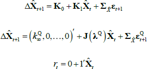
where  is a scalar, J(λQ) is a diagonal matrix,
  is a lower triangular matrix and 1′ is a vector of ones. The nominal part of our model fits within this framework. To incorporate the real part of our model we need to know how the inflation equation (Equation (A7)) maps between the standard and JSZ representations. But Equation (A17) of JSZ shows how to map from JSZ parameters
  to standard parameters (ρ0, ρ1):

where C and D are functions of the model parameters (see also Equations (15) and (16) in Proposition 2 of JSZ). The inflation equation 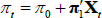 has the same functional form as
  , and so the mapping is given by Equation (B1) also. Reversing the mapping, if one starts with
 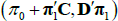 in the JSZ representation, that is
 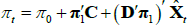 , this maps back to (π0, π1) in the standard representation so that
 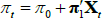 as desired.
The survey data are assumed to be noisy observations on the true underlying expectations for short-term interest rates or the inflation rate. Focusing on the inflation rate (the short-term interest rate case is the same), we have that 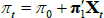 so that
 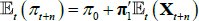 .
.
But iterating forward Equation (A2),  and so we can express the survey data in terms of underlying model parameters (representing true expectations) and some (assumed) normally distributed error term. We include the likelihood of the survey data along with those of the pricing factors and the bond yields in the numerical optimisation. For the case of estimation with observable factors, the survey data is allowed to affect estimates of the parameters but not the factors themselves, as these are constrained to be the principal components of the bond yields (for a yield-only model this is actually no constraint at all, but for a model with surveys it does impose constraints). But in fact, since expectations of short-term interest rates and the inflation rate depend on the future expected value of the pricing factors, the survey data also contains information on these pricing factors. We allow for this in the Kalman filter framework where factors are not directly observable and must be estimated (‘Case F’ in JSZ). This means that we no longer achieve separation of P and Q parameters in estimation, but the dependence is nonetheless relatively weak which, combined with good starting values from the estimation using observable factors, results in a relatively easy-to-estimate model.