RDP 2018-01: A Density-based Estimator of Core/Periphery Network Structures: Analysing the Australian Interbank Market 4. Existing Core/Periphery Estimators
February 2018
- Download the Paper 1,628KB
For any given assignment of banks into core and periphery subsets (henceforth, CP split), the differences between the real-world network and the idealised CP structure create ‘errors’. For example, a link between two periphery banks is an error, as is a missing link between two core banks. Therefore, changing the CP split (e.g. changing a bank's designation from core to periphery) may change the total number of errors.
All estimation methods presented in this section are (either explicitly or implicitly) based on minimising these errors. If the real-world network coincided exactly with the ideal CP structure, the differences between these estimators would not matter (i.e. they would all identify the ideal CP structure as being the CP structure of the network). But since such a scenario is unlikely, each method can lead to a different conclusion.
After describing the key methods available in the literature, we show how their relative performance may depend on the features of the network, such as the density.[15] In Section 4.4, we analytically show how one of the commonly used estimators can be an inaccurate estimator of the size of the core. We then derive a density-based estimator that is immune to the source of this inaccuracy (Section 5). Section 6 numerically evaluates the relative performance of the various estimators (including our new estimator) when applied to simulated networks with the same features as our data. Our estimator is the best-performing estimator when applied to these simulated networks.
4.1 The Correlation Estimator
For any given CP split of a network we can produce both an ideal CP adjacency matrix (Equation (1)) and an adjacency matrix where each of the nodes is in the same position as in the ideal matrix, but the links are based on the links in the data.
Looking only at the core (upper-left) and periphery (lower-right) blocks of the two adjacency matrices, suppose we computed the Pearson correlation coefficient (henceforth, correlation) between the elements of the ideal adjacency matrix and the elements of the real-world matrix. One way to estimate the CP structure of the network is to find the CP split that maximises this correlation.[16] This is the method used by Borgatti and Everett (2000) and Boyd, Fitzgerald and Beck (2006), for example. Specifically, the correlation estimator finds the CP split that maximises the following function:
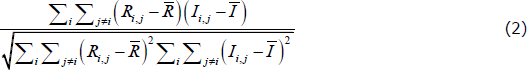
where the sums only occur over elements in the core and periphery blocks, Ri,j is the ijth element in the real-world adjacency matrix,  is the average of these elements, and Ii,j and
  are the equivalent variables from the ideal set.
Each element of the sum in the numerator will be positive if Ri,j = Ii,j (i.e. if there is no error), and will be negative otherwise. It is in this sense that the correlation estimator is an error-minimisation method. With this property, it is tempting to think that the correlation-maximising CP split is also the split that minimises the number of errors. However, any change in the CP split will change the values of , , and the denominator. So the CP split that maximises Equation (2) may not minimise the number of errors.
If the real-world network exhibits an ideal CP structure, then there exists a CP split where the correlation function equals one (the maximum possible value). Therefore, if the real-world network has an ideal CP structure, this structure will be identified by this estimator.
4.2 The Maximum Likelihood Estimator
Wetherilt et al (2010) use a maximum likelihood approach similar to Copic, Jackson and Kirman (2009) to estimate the set of core banks in the UK unsecured overnight interbank market.[17]
Unlike the other estimators outlined in this section, this method makes a parametric assumption about the probability distribution of links within the network; the parametric assumption is a special case of the stochastic block model (Zhang et al 2015). Specifically, for a given CP split, this method assumes that the links in each of the blocks of the real-world adjacency matrix have been generated from an Erdős-Rényi random network, with the parameter that defines the Erdős-Rényi network allowed to differ between blocks. This leads to a likelihood function that is the product of N(N − 1) Bernoulli distributions, as shown in Appendix A.
In Appendix A, we also show that the likelihood of each block is maximised if the elements of the block are either all ones or all zeros. So, if we ignore the off-diagonal blocks, the true CP split of an ideal CP network produces the largest possible value of the likelihood function.[18] Therefore, the likelihood estimator will find the true CP structure if it satisfies the features of an ideal CP structure.
However, while correctly specified maximum likelihood estimators are known to have good asymptotic properties, it is not clear how this estimator will perform against other estimators with real-world networks (especially with N + 4 parameters to estimate, see Appendix A). Even with large unweighted networks, Copic et al (2009, p16) state that ‘there will often be a nontrivial probability that the estimated community structure will not be the true one’. Smaller networks, and CP structures that do not satisfy the estimator's parametric assumption, will likely make this problem worse.
4.3 The Craig and von Peter (2014) Estimator
The Craig and von Peter (2014) estimator (henceforth, CvP estimator) is an explicit error-minimisation method that has been used in multiple subsequent studies (e.g. in ′t Veld and van Lelyveld 2014; Fricke and Lux 2015). This estimator chooses the CP split that minimises the number of errors from comparing the corresponding ideal adjacency matrix to the real-world adjacency matrix:[19]

where, for a given CP split, eCC is the number of errors within the core block (caused by missing links) and ePP is the number of errors within the periphery block (caused by the existence of links).
As noted earlier, an ideal CP structure requires each core bank to lend to and borrow from at least one periphery bank. In the CvP estimator, if a core bank fails the lending requirement, this causes an error equal to N − c (i.e. the number of periphery banks to which the core bank could have lent); borrowing errors are computed in an analogous way. These lending and borrowing errors are captured in eCP and ePC, respectively.
4.4 Theoretical Analysis of the Craig and von Peter (2014) Estimator
An accurate estimator of the true CP structure should not be influenced by the addition of noise. In other words, the existence of some random links between periphery banks, or the absence of some random links within the core, should not systematically bias an accurate estimator. In this section, we evaluate how the addition of noise influences the CvP estimator.
A feature of the CvP estimator is that a link between two periphery banks has the same effect on the error function (Equation (3)) as a missing link between two core banks. At face value, this is reasonable; the ‘distance’ from the idealised CP structure is the same in both cases. But this equal weighting does not account for the expected number of errors within each block, and has important implications for the performance of the CvP estimator.
For example, take a true-core block of size 4 and a true-periphery block of size 36, and start with the correct partition. Moving a true-periphery bank into the core causes a maximum of eight additional errors within the core block (i.e. potential missing lending and borrowing links with the four other core banks). Even if this moved bank had no links with the true-core banks, if it had more than eight links with other true-periphery banks due to idiosyncratic noise (out of 2 × 35 possible links), and these links included at least one lending and at least one borrowing link, moving it into the core would reduce the total number of errors. Therefore, the CvP estimator would overestimate the size of the core in this scenario.
While this is just a stylised example, something like this is actually a high probability event; with even a small amount of noise (e.g. a periphery-block error density of just 0.06), the probability of there being a true-periphery bank with more than eight within-periphery links is over 50 per cent. So, with this CP structure, there is a high probability that the CvP estimator would overestimate the size of the core.
The problem is, that with this CP structure (i.e. when the periphery block is much larger than the core block) even a small amount of noise is expected to produce a sufficiently large number of periphery-block errors that an overestimate becomes the optimal response of the CvP estimator. If, on the other hand, an estimator depended not on the number of errors within each block but the proportion of block elements that are errors, it would implicitly account for the fact that larger blocks can produce a larger number of errors, and would therefore not be subject to the same problem. It is this idea that guides the derivation of our ‘density-based’ estimator in Section 5.
But before deriving our estimator, we must evaluate this problem more generally. To simplify the analysis, we focus only on the performance of the CvP estimator in determining the true size of the core (as opposed to determining which banks are in the core). We focus on the CvP estimator because the simple form of this estimator's error function allows us to analytically evaluate the sources of inaccuracy.
4.4.1 Simplifying assumptions
Our analysis uses three simplifying assumptions:
Assumption 1: Continuum of banks
We assume the network consists of a continuum of banks normalised to the unit interval [0,1]; so each individual bank has an infinitesimal effect on the CvP error function. Therefore, N = 1, and c can be interpreted as the share of banks in the core.
Assumption 2: Banks are representative
We are able to focus on core-size estimation by assuming that any subset of true-periphery banks has the same effect on the CvP error function as any other equal-sized subset of true-periphery banks. In other words, with respect to the error function, each equal-sized subset of true-periphery banks is identical.
We make the same assumption for the true-core banks (i.e. with respect to the error function, each equal-sized subset of true-core banks is identical). Another way to think about Assumptions 1 and 2 is that we have a continuum of representative true-core banks and a continuum of representative true-periphery banks.
Assumption 3: The core/periphery model is appropriate
If a network consists of a true core/periphery structure and ‘noise’, we do not expect the noise to be the dominant feature of the network; if it were to dominate, it would be more appropriate to model what is causing the noise rather than using a core/periphery model. So we assume that the noise does not cause too large a deviation of the network from a true core/periphery structure. Specifically, we assume:

where dC is the density of links within the true-core block, dO is the density of links within the true off-diagonal blocks, and dP is the density of links within the true-periphery block.
With this set-up, noise is added to the ideal CP structure by removing links from the core (i.e. setting dC < 1) and/or adding links to the periphery (i.e. setting dP > 0).
4.4.2 Impact of the simplifying assumptions
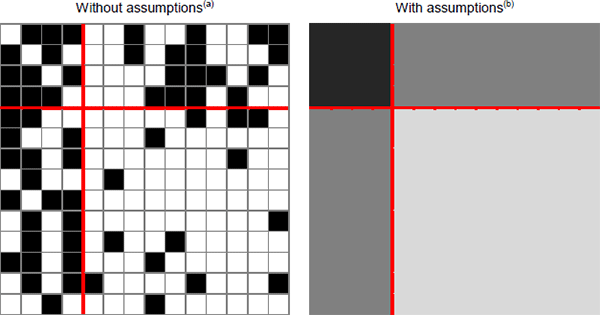
Without these simplifying assumptions, the sorted adjacency matrix of a hypothetical network with a core/periphery structure and some noise would look something like the left panel of Figure 4. As detailed in Section 3.4, each row/column in this matrix represents a bank's lending/borrowing. Banks are sorted so that the banks placed in the core are first; the red lines partition the matrix into the core, periphery, and off-diagonal blocks described in Equation (1). Black cells represent the existence of a link, white cells indicate non-existence.
With our simplifying assumptions, a hypothetical sorted adjacency matrix (with the true CP split identified) would look more like the right panel of Figure 4. This is because:
- Having a continuum of banks (Assumption 1) means each individual bank has measure zero. As a result, individual elements of the adjacency matrix have measure zero; hence the right panel is shaded instead of having individual elements like the left panel. This also means the diagonal elements of the adjacency matrix (i.e. the elements excluded because banks do not lend to themselves) have measure zero. This implies, for example, that there are c2 potential errors in a core block of size c, rather than the c(c − 1) in the integer version.
- Having representative banks (Assumption 2) means the density of links within any subset of true-periphery banks is the same as for any other subset of true-periphery banks; this is also true for the density of links between this subset and the true core. If this were not the case, some subsets would have a different effect on the CvP error function, violating Assumption 2. Analogous reasoning applies to the true-core banks. As a result, the entirety of each true CP block has the same shade.
Notes:
The red lines partition the matrix as described in Equation (1)
(a) Black cells indicate a one in the adjacency matrix, white cells indicate a zero
(b) Darker shading indicates a higher density of links within the block (black represents a density of one, white represents a density of zero)
Without the simplifying assumptions, the CP split is defined by N binary variables (each bank must be defined as either core or periphery). The advantage of having the adjacency matrix look like the right panel of Figure 4 is that the CP split becomes defined by just two variables, the share of banks that are in the true core but are placed in the periphery (x) and the share of banks that are in the true periphery but are placed in the core (y). Denoting the true share of banks that are in the core as cT, then x∈[0,cT], y∈[0,1 − cT], and the share of banks placed in the core (i.e. the CP split) is c = cT − x + y. An accurate estimator of the core will set x = y = 0.
The simplifying assumptions also simplify the CvP error function. With the network parameters {dC, dO, dP, cT}, and the variables {x, y}, the CvP error function becomes:

The components of this simplified CvP error function are best explained using a hypothetical adjacency matrix with an incorrect CP split (Figure 5):
- (1 − dC) (cT − x)2: Errors arising from missing links between the true-core banks placed in the core (in an ideal CP structure, the density of links within the core is equal to one).
- (1 − dO) (cT − x)y: Errors arising from missing links between the true-periphery banks incorrectly placed in the core and the true-core banks placed in the core.
- (1 − dP)y2: Errors arising from missing links between the true-periphery banks incorrectly placed in the core.
- dCx2: Errors arising from links between the true-core banks incorrectly placed in the periphery (in an ideal CP structure, the density of links within the periphery is zero).
- dO(1 − cT − y)x: Errors arising from links between the true-core banks incorrectly placed in the periphery and the true-periphery banks placed in the periphery.
- dP(1 − cT − y)2: Errors arising from links between the true-periphery banks placed in the periphery.
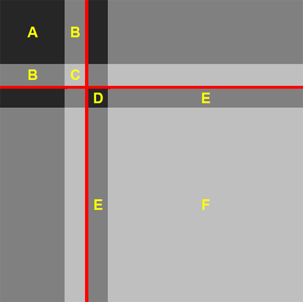
Note: The red lines indicate one possible incorrect CP split
As long as dP > 0, the density of links within any subset of the off-diagonal blocks will be non-zero (as there will be no white shading in Figure 5). As a result, there will be no off-diagonal block errors with any CP split. Allowing for dP = 0 increases the complexity of the error function, so we exclude this unlikely boundary scenario in this section of the paper. Appendix B shows that neither the CvP estimator nor our new estimator permit a core/periphery structure with off-diagonal block errors.
4.4.3 The error-minimising core size
In Appendix B, we prove that for a given c ≥ cT, the value of x that minimises eCvP is x = 0. This means that when the estimated core is at least as large as the true size of the core, no true-core banks will be placed in the periphery. Intuitively, for any c ≥ cT, if a subset of true-core banks is placed in the periphery (i.e. if x > 0), then a subset of true-periphery banks (that is at least as large) must be in the estimated core (recall that c ≡ cT − x + y). But with dC > dO > dP (Assumption 3), the number of errors could be reduced by switching the true-core banks currently in the estimated periphery with some of the true-periphery banks currently in the estimated core (i.e. by setting x = 0 and y = c − cT). Using Figure 5 as an example, this would occur by switching the banks causing errors D and E with the banks causing errors B and C.
Using the same intuition (with proof in Appendix B), for a given c < cT, all the banks that make up the estimated core must be true-core banks (i.e. y = 0). But since c < cT, some true-core banks must also be in the periphery; so x = cT − c > 0 in this scenario.
With the optimal values of x and y determined for any value of c, the error-minimisation problem reduces to one with a single variable (c). Graphically, the CvP estimator sorts the banks so that the shading of the adjacency matrix will look like the right panel of Figure 4 (as opposed to Figure 5), all that is left to determine is where to place the red lines. From this point, the result depends on the values of the parameters {dC, dO, dP, cT} (the results below are proved in Appendix B):
-
When the densities of links in the true-core (dC) and true off-diagonal blocks (dO) are sufficiently small relative to the true size of the core (cT), the CvP estimator underestimates the true size of the core.
- With dC > dO > dP, moving true-core banks into the periphery (i.e. setting c < cT) increases both the density of links within the periphery block and the size of the block; so the number of errors from this block increases. But it also reduces the size of the core block, thereby reducing the number of errors from within the core block (the density of errors within the core block does not change). When dC and dO are sufficiently small relative to cT, the reduction in errors from the core block more than offsets the increase from the periphery block, causing the CvP estimator to underestimate the size of the core.
-
When the densities of links in the true-periphery (dP) and true off-diagonal blocks (dO) are sufficiently high relative to the true size of the core, the CvP estimator overestimates the true size of the core.
- The intuition is analogous to the previous scenario. When dP and dO are sufficiently high and some true-periphery banks are placed in the core, the fall in the number of errors coming from the periphery block more than offsets the increase in the number of errors coming from the core block, causing the CvP estimator to overestimate the size of the core.
- In between these two scenarios, the CvP estimator accurately estimates the size of the core.
To be precise, the CvP error-minimising core size is:
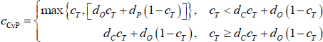
What this means, practically, is that if the density of the network is large (small) relative to the true proportion of banks in the core, the CvP estimator will tend to overestimate (underestimate) the size of the core. Moreover, this inaccuracy will worsen the further the density of the network deviates from the true proportion of banks in the core. This occurs because networks with these properties are expected to generate a large number of errors in one of the blocks, but the CvP estimator does not account for this and instead offsets these errors by changing the size of the core.
Footnotes
While our paper is the first to assess the relative performance of these estimators, in ′t Veld and van Lelyveld (2014, p 33) mention that with the estimator they use the ‘relative core size is closely related to the density of the network’ and that ‘one should therefore be careful not to take the core size too literally’. [15]
Since these sets do not incorporate the off-diagonal blocks of the adjacency matrices, this method does not require an ideal core bank to be an intermediary. [16]
Variations of the maximum likelihood estimator are also used in the literature, see Chapman and Zhang (2010) and Zhang, Martin and Newman (2015), for example. [17]
We follow Wetherilt et al (2010) and include the off-diagonal blocks in the likelihood function. This improves the performance of the maximum likelihood estimator in the numerical analyses conducted in Section 6. We note, however, that in small samples the theoretical implications of including the off-diagonal blocks in the likelihood function are not clear. [18]
Craig and von Peter (2014) actually minimise a normalisation of this error sum. However, this normalisation is invariant to the CP split, so it can be ignored for our purposes. [19]