RDP 2014-06: Is Housing Overvalued? 7. Sensitivity

Our baseline results apply to national averages. Potential home buyers will wish to vary these estimates depending on their individual circumstances and judgements. In some cases, this is simple: for example, a household expecting lower running costs or borrowing at a lower-than-average mortgage rate would see their user cost decline one-for-one. In the following sections we discuss two variations that are less straightforward: the expected rate of capital gains (Section 7.1) and the period for which a house is expected to be owned (Section 7.2).

7.1 Capital Appreciation

Figure 5, which shows several measures of house prices, highlights some of the uncertainty about capital appreciation and the range of plausible assumptions. Of particular interest are the estimates of constant-quality prices constructed by Nigel Stapledon in orange, with median house prices in dark blue. As discussed in Appendix A, Stapledon's constant-quality estimates provide a useful focal point – in part because they are more clearly consistent with other elements of the user cost than other house price measures.

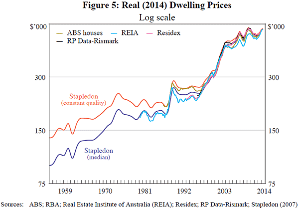
Two observations are worth noting. First, real constant-quality house prices have trended up steadily since the 1950s. Figure 5 uses a log scale to show the similarity of growth rates in different periods. Growth in the second half is slightly faster than in the first half, but the difference is small both in economic terms and relative to the noise in the data. To be more precise, the series resembles a random walk with relatively constant drift. Second, other data series are available over shorter periods, but show similar trends.

Because real house prices in Australia have continued to rise over a long period of time, induction suggests that this trend will continue. The mean of a long sample provides a simple and transparent first approximation to what should be expected in the future.

However, trends need not be stable. Some observers (e.g. the Financial Stability Review (RBA 2013, p 50) and Ellis (2013)) suggest that capital appreciation in the future may be lower than in the past. Accordingly, Figure 6 shows some alternative benchmarks that house prices might be expected to follow. The blue line shows how estimates of overvaluation would vary accordingly.

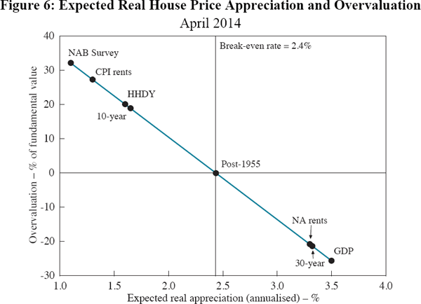
The 10-year and post-1955 averages shown in Table 1 have been discussed above. The 30-year average, a benchmark referred to by Ellis (2013), is conceptually similar. Real disposable income per household (labelled ‘HHDY’) has grown at an average annual rate of 1.6 per cent since 1960. Were house prices expected to grow at this rate, housing currently would be approximately 20 per cent overvalued. A limitation of this measure is that it excludes population growth. Broader measures of income, such as real GDP, which may be better proxies for overall housing demand, have grown at an average rate of 3.5 per cent since 1960, implying undervaluation. A more theoretically attractive assumption is that house prices grow in line with rents; but again, different measures are available. Real rents measured by the CPI have risen 1.3 per cent since 1960. Real gross rents per dwelling, based on the national accounts (labelled ‘NA rents’), have risen an average of 3.3 per cent.^[5]

Forecasts of future price growth should encompass the above measures together with other relevant information. One set of forecasts comes from the 2014:Q1 NAB survey of property professionals, whose respondents project that house prices will rise 2.8 per cent over the next year. It is unclear what definition of prices respondents have in mind, but we suspect it is the price for a ‘given house’, which includes wear and tear but excludes improvements. To make this comparable with other estimates, we add our assumption of physical depreciation (1.1 per cent, discussed in Section A.3) and subtract expected inflation (2.8 per cent, discussed in Section A.7), to give an expected rate of real appreciation of constant-quality houses of 1.1 per cent. Were this rate of appreciation to continue, it would imply overvaluation of 32 per cent. The NAB survey provides a direct measure of expectations, which is useful for many purposes, such as analysing buyer behaviour. However, for reasons we discuss in Appendix A.2, it does not seem a reliable indicator of future price changes.

Expectations of professional forecasters avoid some of the problems of the NAB survey.^[6] However, averaging these forecasts is difficult, partly because some deserve more weight than others. That said, our judgement is that the central tendency of published house price forecasts is probably for moderate real appreciation over the next few years, at a somewhat slower rate than the long-term historical average. This would imply that houses are slightly overvalued. However, there are also reputable forecasts that imply undervaluation, fair valuation and substantial overvaluation.

It could be assumed that the predictions of a well-specified econometric model would appropriately summarise the available information and provide a plausible measure of expectations, or at least, what they should be. However, it is not clear that statistical models provide a plausible basis for decision-making. For example, Garner and Verbrugge (2009) estimate a variety of time series models for US house prices. These models often imply very strong expected appreciation, which in turn implies negative user costs. It is doubtful that US households, as a group, did or should have acted on the assumption that the cost of buying a house was negative. It may be that the accuracy of the models was impaired by the short samples for which some explanatory variables were available.

7.2 Length of Tenure

Home ownership is more attractive the longer a house is owned, because transactions costs are amortised over a longer period. However, because housing tenure affects the user cost non-linearly, the size of this effect is not obvious. We show break-even appreciation rates for varying lengths of tenure in Figure 7. Because issues of timing seem central, we use the discounted cash flow model of Section 5.4.

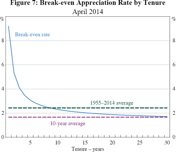
With historical average real house price expectations of 2.4 per cent, represented by the green dashed line in Figure 7, buying is less expensive than renting for anyone expecting to stay in their house for more than eight years. This contrasts with a threshold of ten years using the static model. If real appreciation over the previous 10 years (1.7 per cent) is used as a guide (the purple dashed line), buying is less expensive than renting only with extremely long expected tenure (in excess of 30 years). Consistent with conventional wisdom, households expecting to move again in a few years' time are better off renting, unless they believe they can sell the property for an unusually large capital gain.

Footnote

Estimates of rents are from Stapledon (2007), kindly updated by Nigel Stapledon. There are concerns that the CPI measure has too large an adjustment for quality changes. The national accounts measure is not quality adjusted. An estimate of rental growth consistent with our measure of price appreciation would probably lie between these estimates. [5]

A convenient source for private sector forecasts of property prices is www.propertyobserver.com.au. One of the most widely cited forecasts is that of BIS Shrapnel, reported in Schlesinger (2013). [6]