RDP 2011-04: Assessing Some Models of the Impact of Financial Stress upon Business Cycles 6. Correspondence of GOZ Model Business Outcomes with Stylised Facts
December 2011
- Download the Paper 265KB
We now seek to examine some of the characteristics listed in Section 3. In order
to compare the model's output with the stylised facts, it will be necessary
to find the credit growth rates implied by the model. Appendix A shows that
the growth in real debt,  equals
where γ is the long-term rate of growth of per capita output, lt is leverage and an asterisk indicates these are measured in percentage form.
6.1 Credit and Output Growth Following a Financial Crisis
To assess the first relation documented by the IMF using simulated data we computed
GDP growth and real credit growth over the first eight quarters of expansions.
Let these be Δzj and Δcj respectively, where
j indexes an expansion. Forming ϕj = Δzj
− Δcj, the stylised facts would be that the
average of ϕj from expansions that come after
a financial crisis would be positive. Given that we use the size of the external
finance premium  as an index of the extent of a financial crisis, we would expect some relation between
ϕj and ψj, where
ψj is the external premium when the j′th
expansion began. We used three measures of ψj : the
value of the premium at the origin of the expansion (at time tj),
and two averages based on current and past values,
  and
and  . As the conclusions were the
same in all cases we present the relation with the first of the three measures.
Then the regression of ϕj upon ψj
and a constant gives (with t-statistics in parentheses)
suggesting that credit growth is increasingly weaker than output growth over the first two years of expansion when the external premium at the beginning of the expansion is larger.
It is worth noting that the average credit growth over the first eight quarters of all expansions is 0.6 per cent versus the 4.3 per cent in output. But this hides an enormous variation. There are many simulations in which the growth in credit over the first two years of an expansion exceeds that of output. This remains true for a significant number of expansions which are preceded by a high external finance premium, which we would interpret as a financial crisis. The growth rates in credit are extremely volatile, with a standard deviation of quarterly growth of 3.68 versus only 0.66 for output, although this volatility is also in the actual data used by GOZ.[11]
6.2 Recessions and Financial Crises
We can investigate the dependence of recessions upon the external finance premium
by taking advantage of the binary nature of the recession indicator Rt(Rt = 1 if the economy is in recession
but zero otherwise). One possibility is to compute the probability of a recession
as the external finance premium rises;  . Assuming this has a Probit
form it will be
  ,
where
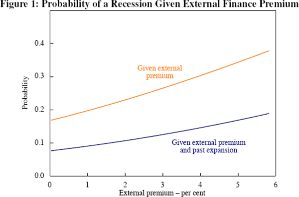
  is the cumulative standard normal distribution function. Figure 1 plots this as
a function of st from simulations of the GOZ model. Note
that the unconditional probability of an NBER recession over 1953:Q2–2009:Q4
was approximately 0.16. While the rise in the external premium does increase
the probability quite substantially, it never gets to a standard critical value
often used in predicting recessions of 0.5.

An alternative indicator of the relationship between recessions and the external finance premium comes from recognising, following Harding (2008), that the recession states Rt generated by BBQ (and also true for NBER recession indicators) follow a recursive process of the form
where ∧t is a binary variable taking the value unity if a peak occurs at t and zero otherwise, while ∨t indicates a trough. By definition ∧t = (1 − Rt)Rt+1 and ∨t =(1 − Rt+1)Rt. In BBQ,
where Δ2yt = yt − yt−2 will be six-monthly growth. Then one might condition upon the previous states as well as the external finance premium, to determine what the probability of going into a recession at time t is for a given finance premium and the knowledge that we were in expansion at t − 1 and t − 2. This probability, using Equation (8), will be
where the conditioning on the past expansions has been suppressed. Assuming a Probit
again, Figure 1 contains a plot of this against  .
There is clearly a big difference between it and
  . If it is known that one is
in an expansion in the preceding two periods the rise in the probability of
a recession, even for large values of the external finance premium, is quite
small. Indeed, the result suggests that the external finance premium will not
be very useful for predicting recessions, a point we come back to later.
6.3 The Duration of a Recession and the Size of the External Finance Premium
The next question we seek to examine is whether the duration of recessions depends
upon the magnitude of the external finance premium. There are two ways one
might do this. One is to relate the durations of recessions to the external
premium. To do this, we simulated a long series of data and regressed the durations
of recessions in this series against the external finance premium at the beginning
of the recession. While this showed a positive relationship the connection
was not strong – even large changes in the premium only caused the duration
to increase by just a quarter. Another method is to compute  ,
i.e. the probability that, in m periods time, the economy will still be in
a recession given it was in recession at time t, conditional on the
external finance premium. Table 3 shows what this probability is for three
levels of
  and for m = 2,3,4. This probability effectively is a measure of duration
dependence.
External premium  (basis points) (basis points) |
m = 2 | m = 3 | m = 4 |
|---|---|---|---|
| 25 | 0.51 | 0.36 | 0.27 |
| 300 | 0.53 | 0.37 | 0.28 |
| 485 | 0.53 | 0.38 | 0.29 |
It appears that the probability of a recession continuing only increases slightly with a larger initial external finance premium. Essentially, both computations address the often-quoted result that a recession associated with a financial crisis is around twice as long as one that does not have one. While we would think that a crisis would involve a high external interest rate premium, given that there would be little credit available, the GOZ model only delivers such a prediction in a very weak way. One would certainly associate a crisis with an elevated probability of recession, as seen in Figure 1, but its duration does not seem to depend much on the premium. One factor contributing to this might be the persistence in the growth in credit; the persistence in {Δln(1 − (1/lt))}, which is used to form credit growth in Equation (7), is considerably smaller in the model than in the data.
6.4 Credit Growth and Recession Prediction
One might ask if there is any evidence that a recession can be predicted with the
GOZ model. The probability is different to what was computed above as we are
now looking at  and not
  .
We might also be interested in
  . The latter equals
pointing to the fact that predicting a recession involves successfully predicting negative quarterly and six-monthly growth over the two quarters following on from the prediction point. This is much stronger than the ability to predict growth rates of output per se. It may be that we predict positive ones quite well, and this can make the prediction record for output growth look rather good, even though recession prediction is a dismal failure.
There are some current difficulties in determining the predictions of the GOZ model
since it was estimated using some data that were not available to us. In particular,
the credit spread was one they constructed. To gain an idea of how useful the
model might be we assume that the latter is well represented by the Baa
spread.[12]
The figures in GOZ suggest the Baa spread is related to their indicator, although
they argue that their measure is a better predictor. With the Baa spread as
 we evaluate
  .
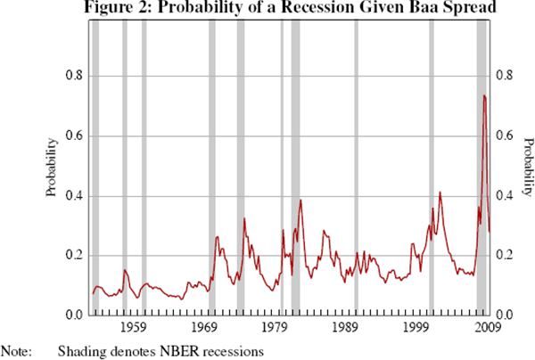
Here the Baa spread used is that available at the beginning of the quarter
for which a prediction is to be made. Although the spread is significant in
a Probit model fitted to the recession indicator (t ratio of 3.5),
it is clear from Figure 2 that it adds little to the predictive power. Even
in 2008, it was not indicating a recession until the recession was well under
way (the predicted probability in the first quarter of 2008 was just 0.23).
This concurs with the finding of Harding and Pagan (2011) that many series
recommended as useful for predicting recessions in fact have little predictive
power, and suggests that the external finance premium, a key part of the GOZ
model, might be ineffective at predicting
recessions.[13]

To understand the limits of using models such as this for predicting recessions we
observe that, at time t − 1, we would be predicting 1(Δyt
< 0,Δ2yt+1 < 0) using the
information available at t − 1, that is, we aim to predict future
growth outcomes. A check on whether a model would be able to predict such a
quantity is to ask how important the unpredictable part of future shocks are
to these growth outcomes. Shocks, such as technology, often have an autoregressive
structure, and it is the innovation whose impact upon the business cycle we
wish to determine. We therefore simulate the GOZ model turning off the contemporaneous
innovations, that is, the model is run with the current innovations set to
zero, although they are re-set to their actual values in later periods. To
illustrate what is done, take an  , where et is white noise.
Defining
  ,
we note that zt and
  differ only in that the current
innovation is set to zero; in other words,
  is the predicted value of
zt. Table 4 shows the business cycles from the GOZ model
with current innovations present (equivalent to basing the computation on zt)
and with them suppressed (equivalent to
  and hence designated GOZ−).
It is clear that the current innovations have an enormous effect upon the cycle
characteristics. Abstracting from current innovations, expansions now become
very long, and so there will be fewer recessions, leading to our conclusion
that the GOZ model will predict fewer recessions if future shocks are not known.
| GOZ | GOZ− | |
|---|---|---|
| Durations (qtrs) | ||
| Expansions | 14.8 | 33.9 |
| Contractions | 4.2 | 4.2 |
| Amplitude (%) | ||
| Expansions | 9.0 | 15.9 |
| Contractions | −1.6 | −0.8 |
| Cumulative amplitude (%) | ||
| Expansions | 107.9 | 461.8 |
| Contractions | −5.2 | −2.8 |
| Note: GOZ− is the GOZ model with current innovations to shocks supressed | ||
6.4.1 Relative performance of investment prediction
One of the observed cycle characteristics listed above was that there would be a
stronger response by investment than output. We therefore studied the investment
cycle present in the observed investment data used by GOZ, namely a chain-weighted
index of per capita private fixed investment and durable goods. Here expansions
were 12 quarters long on average and contractions were 6.5 quarters. So, while
the investment cycle length is not far from that of GDP, the contractions are
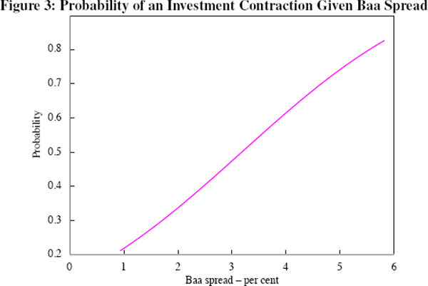
longer and the expansions are shorter. Figure 3 presents the probability of
an investment recession as a function of the Baa spread,  ,
and it is apparent that it rises very quickly with the spread. This is also
true of the model, where the probability of an investment contraction is 0.47
when there is an (annualised) spread of 205 basis points, 0.58 when the spread
is 305 points, and 0.78 when it is 515 basis points.

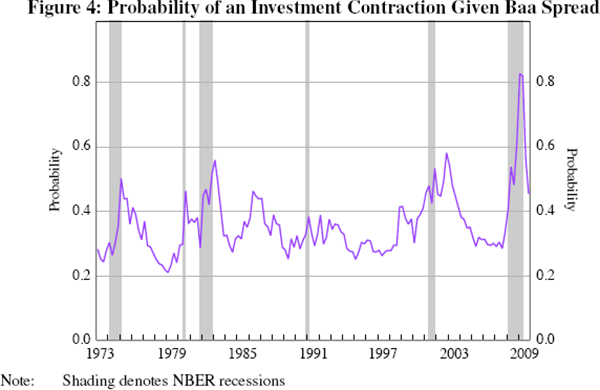
Figure 4 shows the probability of an investment contraction given the Baa spread over the GOZ estimation period. A comparison with Figure 2 suggests that the probability of an investment recession tends to be higher than that of output recessions for a given spread, reflecting in part the fact that investment is only one component of output, and therefore a very large negative growth rate in investment is needed to cause a decline in output by itself. This is the case in the GOZ model; despite using a relatively wide definition of investment in estimation, the parameters of the model (in particular α, which governs its weight in the production function) imply a steady-state investment-to-output ratio of around 6.5 per cent, which is less than fixed non-residential investment's share of output in the data. If α is doubled then the model matches the business cycle characteristics of the data better and the effects of an increase in the external finance premium are greater. For example, an increase in the external finance premium from 25 to 300 basis points raises the probability that an economy in recession now will remain there two quarters in the future from 0.51 to 0.57, which is still a small increase but more than double the impact shown in Table 3. Similarly, the probability of a recession at large values of the external finance premium is higher, but remains below 0.5.[14] As the role of investment in the GOZ model is more aligned with fixed non-residential investment, increasing α much further is not realistic. In all, it appears that one needs to work with a broad set of investment expenditures, i.e. housing and consumer durables could be important to getting the quantitative financial effects right and these probably should be integrated into the structure of the model. In turn this implies that collateral effects might be important.

Footnotes
The extreme volatility comes from the factor  in the growth of credit as set out in Equation (7). If one computes the standard
deviation of
  from the data and the model we find these to be 5.53 and 4.89 respectively.
[11]
Because there are two interest rates in the model, and one of these is the policy rate, it might be better to use the spread over a three-month Treasury bill rate. But doing this does not change the results very much. The Baa spread is calculated using data from the Federal Reserve Board of Governors Statistical Release H.15. [12]
We also experimented with using the GOZ model itself to predict recessions, that
is, we constructed an estimate of  from the GOZ model, where Ft denotes the information set from
the model excluding the external finance premium (i.e. we delete its influence).
Then
  and the Baa spread were both used in the Probit model. Each variable was significant
but there was no improvement in predictive power for recessions over that
shown for the Baa spread.
[13]
At 5 per cent it is approximately 0.42. [14]


