RDP 2010-03: Modelling Inflation in Australia 3. Estimation

The estimation of these models raises a number of challenges both in terms of the dependent variable, the functional form (for example, the lag structures used in the regressions and the modelling of expectations) and the choice of particular variables used in the regressions.

3.1 Data

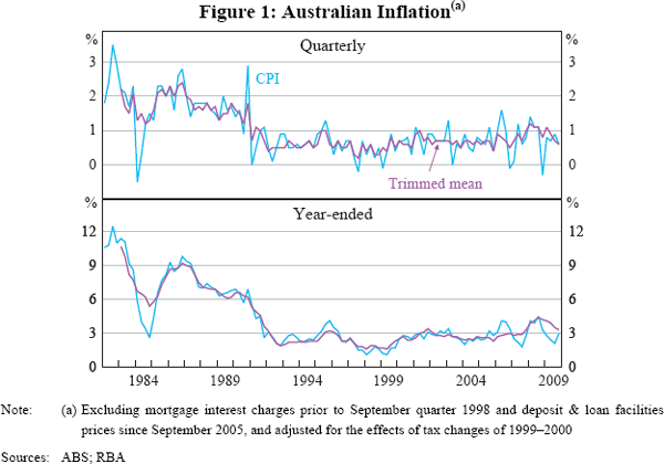
Empirical papers on inflation in different countries typically use headline measures of inflation (based on either the consumer price index or the household consumption price index). Instead, we use an underlying measure: quarterly trimmed mean inflation, where 15 per cent (by weight) of the CPI is trimmed from the upper and lower ends of the distribution of seasonally adjusted price changes in each quarter.^[4] This measure is preferable to headline CPI since it provides a measure of underlying inflation that abstracts from much of the noise in CPI inflation (Figure 1; see also Brischetto and Richards 2006).

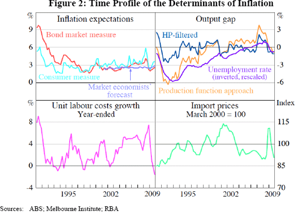
Our measure of inflation expectations is derived from pricing in the bond market, and is calculated as the difference between standard and indexed bond yields at a maturity of approximately 10 years. (Alternative proxies are considered in Section 5.2, and some candidate measures are shown in Figure 2.) There are problems with this measure, including the fact that it includes any shifts in liquidity premia, its long duration (ideally we would use a one- or two-year-ahead expectation) and the fact that it is not directly observed from financial prices prior to 1993 (see Gruen, Robinson and Stone 2002).^[5] However, there are no obviously superior measures and it proves to have some empirical explanatory power.

We estimate nominal unit labour costs as total labour costs divided by real GDP; we use this in preference to the measure published by the ABS which is affected by volatility in the estimate of self-employed income. For real unit labour costs, we deviate from the practice in some of the US literature of using labour's share of total income, given the substantial influence that commodity prices have on the GDP deflator (and hence labour's share) in Australia. Instead, we calculate real unit labour costs by deflating nominal unit labour costs by trimmed mean inflation.

Data on import prices are in local currency and are sourced from the ABS balance of payments release, but are adjusted in three ways. First, we remove ‘lumpy’ imported goods (large one-off imports such as civil aircraft) and oil (due to its volatility) from the calculation to produce an underlying measure of import prices that is more likely to be representative of persistent economy-wide import prices. Second, as in some earlier papers, we remove automated data processing equipment imports due to concerns about the treatment of quality changes when measuring the prices of such imports. Third, we adjust the across-the-docks import price data to include the effect of changes in tariff rates.

Estimates of the output gap are based on a production function approach, in line with the practice favoured by the Organisation for Economic Co-operation and Development (OECD); although, broadly similar results are obtained when we use the capacity utilisation measure from the National Australia Bank business survey or a Hodrick-Prescott filtered output gap. The production approach calculates potential output growth as the weighted average of smoothed growth in the net capital stock and labour inputs (where the weight on each is the capital and labour share of total factor income, respectively) plus smoothed growth in multifactor productivity. This potential growth rate is then converted to a level of potential GDP by assuming that potential GDP was equal to actual GDP on average between 1998 and 2001 (in other words, that the output gap averaged zero over this time); the latter assumption has no effect on the regression results since the output gap is demeaned in each case.

Data for all these variables are sourced from the ABS, with the exception of trimmed mean inflation, which is from the RBA, and inflation expectations, which are from the RBA since 1993 and Gruen et al (2002) prior to that.^[6] All data are included in log or log-differenced form, except the unemployment rate which is in levels.

The main estimation period is from the March quarter 1990 to the December quarter 2009. The rationale for excluding data prior to 1990 is that a priori there is the possibility of a structural break around the disinflation of the early 1990s and the introduction of inflation targeting in 1993. We find evidence in support of this (see Section 6), with rolling Chow tests clearly signalling a break in our inflation equation around March 1989 (particularly in the standard Phillips curve model). The decision to include data from 1990 rather than 1993 reflected a desire to use a slightly longer sample, including the recession at the start of the 1990s, which may improve our ability to accurately estimate coefficients.

3.2 Equation Specifications

The main choices regarding the specification are the appropriate econometric technique to use when estimating each equation, and whether to impose any constraints on the coefficient estimates. There are also questions about the appropriate specification of the lag structure for the right-hand-side variables. In particular, given that several of the variables are likely to feed through into inflation with relatively long lags, it is necessary to consider lag structures which preserve degrees of freedom.^[7]

The approach we use is to estimate each model using various permutations, including in the way that lag structures are modelled. However, for simplicity, we present results from only one econometric specification for each type of model. Having decided on a method to preserve degrees of freedom, the exact lag length and whether to allow speed limit effects or not were chosen by minimising the Akaike information criteria (AIC).^[8]

Using this approach leads us to adopt the following standard Phillips curve specification:

where the coefficients on import prices (γ_k) are constrained to follow a quadratic polynomial function in order to preserve degrees of freedom. The inverse of the unemployment rate is included on account of it both providing the best fit and being theoretically consistent with an increasing effect on inflation from a given change in unemployment as it declines. Given the fact that the unemployment rate is reasonably persistent (both in level and four-quarter-change form), there is a range of feasible lag selections which yield broadly similar results: here we include the unemployment rate with a two-quarter lag as suggested by the data (which may reflect the presence of nominal rigidities in both wage- and price-setting) and a lagged speed limit term as well. We include the prior period's expectation of future inflation to prevent estimation problems associated with endogeneity. Up to three years of lags of import price growth are selected by the AIC.^[9] Lagged inflation is not found to be significant in this model and so is excluded from the estimation.

We estimate the NKPC using the GMM approach, as in Galí and Gertler (1999).^[10] As instruments, we use four lags of inflation and two lags of real unit labour costs. We include only the current observation of the driving variables, so that our final specification is as in Equation (3). We also estimate the NKPC using direct measures of inflation expectations and ordinary least squares (OLS), as per Henzel and Wollmershäuser (2008), in order to avoid having to instrument for inflation expectations. For this specification, we include the prior period's expectation of future inflation and the first lag of all other variables to prevent endogeneity, and we do not constrain the coefficients on inflation and inflation expectations as per Equation (3), so that the specification is:

The main decision when estimating the mark-up model is which econometric specification to use. An error correction specification has been popular in the past, given the theoretical long-run link between the price level and marginal costs. But, as discussed in Stone, Wheatley and Wilkinson (2005), it is difficult to determine whether a cointegrating relationship exists between the price level, unit labour costs and import prices without including another trending variable. Given this, our preference is for distributed lag-type models. Within this class of models, we investigate constraining the coefficients on input costs using either successive four-quarter averages (as in Gordon 2005) or a polynomial distributed lag (PDL) specification (as in Brayton et al 1999). We also estimate the coefficients without any constraints. While the data provide mixed results on the validity of these constraints, we are wary of over-fitting the data (which can occur with the unconstrained model) and the constrained specification provides impulse responses that are easier to interpret. Accordingly, our preferred specification of the mark-up model is:

where the coefficients λ_j and γ_k are constrained to follow a quadratic PDL function. Lagged inflation is found to be insignificant in this specification and so is excluded, and while the change in the output gap is significant at the 10 per cent a level, its coefficient is negative and so we exclude it from the equation.

Footnotes

The measure of trimmed mean inflation is based on data which are adjusted for the impact of the tax changes of 1999–2000. Mortgage interest charges are omitted from the calculation of the trimmed mean prior to September 1998, and the deposit & loan facilities item is excluded from 2005. [4]

Prior to 1993, inflation expectations are estimated as the nominal bond yield less an assumed real bond yield based on data for other OECD countries (see Gruen et al 2002). [5]

Import prices are from the balance of payments release (ABS Cat No 5302.0); total labour costs and GDP are from the quarterly national accounts release (ABS Cat No 5206.0); and estimates of the capital stock and MFP are interpolated from the annual estimates published in ABS Cat No 5204.0. [6]

Approaches used in the inflation modelling literature include: (i) estimation of an unconstrained lag structure, with insignificant lags omitted based an on information criterion or some other testing strategy; (ii) inclusion of long lags but constraints on some of the coefficients to be the same, an approach followed by Robert Gordon in a number of papers, among others; and (iii) the assumption that lag coefficients follow a polynomial function (or Almon lags). [7]

The AIC was used in preference to the Schwarz Bayesian information criterion – which more heavily penalises additional parameters – since we are more interested in finding the best-fitting model than in parsimony. [8]

The appropriate number of lags of imports prices was chosen prior to imposing the polynomial constraint, in order to ensure that the constraint itself did not influence the number of lags. [9]

Rudd and Whelan (2005) criticise the use of GMM on the grounds that any instrument used to proxy future inflation is plausibly correlated with an omitted variable and could therefore bias the estimated coefficients. However, this claim is disputed in Galí, Gertler and López-Salido (2005) and it is still common to use the GMM approach. [10]