RDP 2008-09: A Term Structure Decomposition of the Australian Yield Curve 4. Data and Model Implementation

Estimation of the model presented in Section 3 requires observations of zero-coupon bond yields. As zero-coupon bonds are not currently issued in Australia, we need some way to infer these yields from coupon-bearing Australian Government bonds.

We estimate zero-coupon bond prices from coupon-bearing Australian Government bond data using a modified Merrill Lynch Exponential Spline (MLES) methodology.^[9] This amounts to estimating a risk-free discount function, which we take as a linear combination of hyperbolic basis functions.^[10] As the estimation of the zero-coupon yield curve is not the primary focus of this paper we provide the technical details and a discussion of the issues involved in Appendix A rather than in the main text. A number of different zero-coupon estimation methodologies were considered, with the MLES method chosen due to its ease of implementation and goodness-of-fit.

To estimate the risk-free zero-coupon yield curve at the short end, we use Treasury notes when they are available and OIS rates with maturities less than or equal to 1 year when Treasury notes are not available.^[11] For maturities longer than 18 months we use the yields of Australian Government bonds. Bonds with shorter maturities can become quite illiquid, and tend to suffer from pricing anomalies. We calculate zero-coupon rates at terms to maturity of 3 and 6 months, as well as for 1, 2, 4, 6, 8 and 10 years. The data are sampled at weekly intervals between July 1992 and April 2007.

We supplement these data with survey forecasts of the cash rate and the 10-year bond yield.^[12] The cash rate forecast data are roughly monthly and are available from March 2000 to April 2007 for forecast horizons from 1 to 8 quarters. These forecasts are not available every month, or at all horizons when they are available; the majority come after March 2002 and are for horizons out to 1 year. The 10-year bond yield expectation data are monthly, run from December 1994 to April 2007, and are for horizons of between 3 months and 10 years. In addition to their helpfulness in identification as discussed above, survey data have been shown to counteract many small sample problems (including different parameter sets giving similar model outputs, the mean reversion of latent factors being too fast, and imprecise estimates). Although survey data give average expectations, not the marginal investor's expectation, this is unlikely to be a major problem. In fact survey data have been found to greatly improve accuracy and stability in model estimation.^[13]

Since the pricing equation, Equation (6), requires knowledge of the latent factors, which are unobservable, these latent factors need to be estimated along with the parameters of the model. This is done via the Kalman filter. Using Equation (6), we can write the zero-coupon yield as implied by the term structure model at time t, for a bond maturing at time t + τ, as

where a_τ = α_τ/τ and b_τ = β_τ/τ are both functions of ρ, Σ, λ₀ and (K + ΣΛ). Our term structure implied zero-coupon yields should match the zero-coupon yields we have estimated using traded government bond and OIS rates, however, and so for each observation occurring at time t we can then stack the versions of Equation (7) corresponding to each maturity, τ, as follows

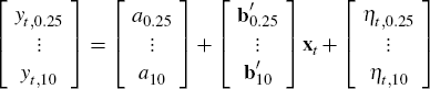
or in matrix notation

Here y_t gives the observed zero-coupon yields, and the error term η_t occurs because our term structure model implied yields a + Bx_t will not fit the observed yields exactly. Note that because the a_τ and are functions of (K + ΣΛ), Equation (8) on its own does not help us separate expected future short rates (determined by K) from term premia (determined by Λ).

We can use the discrete version of Equation (2), however, to write the state equation for the latent factors x_t as

where in our case h = 7/365 (to account for weekly sampling of the data) and 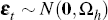with 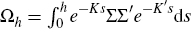.^[14] In Equation (9) K appears on its own, and so with estimates of the latent factors x_t we can infer information about K separate from Λ.

On dates for which there are survey forecasts, Equation (7) changes slightly. Using Equations (1) and (9) we can express cash rate forecasts as

where: τ is the length of time between t and the forecast date; is the cash rate forecast; and denotes the forecast error. Similarly, for bond yield forecasts we can write

where: is the yield forecast; and denotes the forecast error.^[15] Note that in both Equations (10) and (11), K appears on its own, which helps us identify K and Λ separately.

Incorporating the forecast data into our estimation, we can stack Equations (8), (10) and (11) to give the observation equation

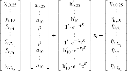
or in matrix notation

To summarise, Equations (12) and (9) then make up the Kalman filter observation and state equations, respectively. These can be used to compute the maximum likelihood estimate of x_t and the parameters ρ, Σ, λ₀, Λ and K, using the zero-coupon yield data and survey data, which together constitute . See Appendix C for further details. As mentioned earlier, K enters our equations separately from Λ via the dynamics of x_t, given by Equation (9), and via the survey forecasts as given in Equation (12).

To estimate the parameters of the model we randomly generate a vector of starting parameters, specify the starting values of the latent factors x_t, and then use the MATLAB^® fmincon function to search for a log-likelihood maximum. The search is based on a sequential quadratic programming routine. This is repeated 2,000 times and the set of parameters producing the highest likelihood is chosen.

This estimation procedure is displayed graphically in Figure 1. One at a time, each of the 2,000 randomly generated sets of initial parameters are fed into the optimisation routine. The routine uses the initial parameter guess to construct the parameters used by the model, such as a and B. Using the Kalman filter, the yield data are used to estimate the latent factors and model implied yields. The Kalman filter also produces the log-likelihood, which the optimisation routine uses to choose a new set of candidate parameters, and the procedure is then repeated. Once the optimisation routine has ended, the highest log-likelihood and the associated parameter values are stored, and the process begins again. After 2,000 iterations, the parameters that produced the highest overall log-likelihood value are chosen.

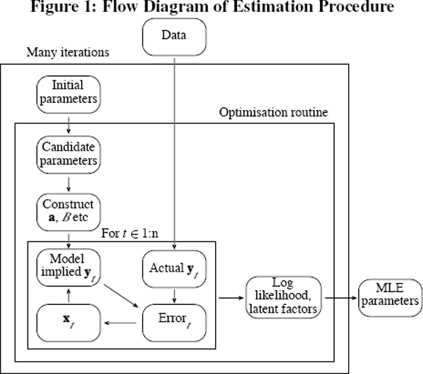
A number of alternative optimisation procedures are possible. We explored simulated annealing, as well as some other in-built MATLAB^® functions, but found that the procedure described above gave the best (highest likelihood values in reasonable time) results.

Finally, from Equation (9) we have 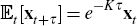, so that having estimated the parameters and latent factors of the model, using Equation (1) we can calculate for time t the expected future short rate (efsr) at time t + τ as

Similarly, from Equation (5) where we are now considering x_t under the risk-neutral probability distribution, for K^* = K + ΣΛ and we have that (see, for example, Kim and Orphanides 2005).

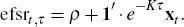
Hence at time t, the model implied forward rate (fr) for time t + τ in the future is given by

But the forward rate at time t applying at time t + τ in the future consists of expectations of the cash rate at time t + τ plus the term premium. Hence, our estimate at time t of the term premium (tp) associated with borrowing or lending at time t + τ in the future is given by

Footnotes

Our modification of the MLES procedure results in the 1-day yield being fixed at the target cash rate. See, for example, Bolder and Gusba (2002) for a discussion of competing estimation methodologies. [9]

The discount function evaluated at t gives the value today of 1 unit at time t in the future. [10]

OIS contracts are over-the-counter derivatives in which one party agrees to pay the other party a fixed interest rate in exchange for receiving the average cash rate recorded over the term of the swap. As no principal is exchanged these contracts are virtually risk-free, and so the fixed rates paid are a good approximation of the average cash rate expected to prevail over the life of the contract. Hence they can be used in place of Treasury notes to estimate the short end to the risk-free yield curve. See RBA (2002) for details of how OIS contracts operate, and Appendix A for more discussion on OIS rates. [11]

The cash rate forecast data are compiled from Bloomberg, Reuters and Consensus Economics, while the 10-year yield forecasts come from Consensus Economics. [12]

See Kim and Orphanides (2005) – they compare models that use and do not use survey data, and perform Monte Carlo simulations on the effect of survey data, finding that survey data counter many of the small sample problems just discussed (note that we use surveys of cash rate expectations and bond yields, whereas they use surveys of the expected yield on US Treasury notes). [13]

Ω_h can be evaluated as . See Kim and Orphanides (2005). [14]

Here we treat a yield to maturity as a zero-coupon yield. Analysis of historically observed yield data shows that the observed yield to maturity on a 10-year bond and the estimated 10-year zero-coupon yield are in fact very close, so this should not be a problem: the difference between the two yield measures is symmetric about zero and has an average absolute size of only 4 basis points. This is less than the precision of the forecast data, which is only reported to the nearest 10 basis points, and well below the forecast error of 50 basis points per square root year that we have assumed (see Appendix C for technical specifications of the model implementation). [15]