RDP 2005-11: A Small Model of the Australian Macroeconomy: An Update 2. Equations
December 2005
- Download the Paper 628KB
The model's six behavioural equations continue to be estimated separately by ordinary least squares (OLS).[8] The equations exhibit no simultaneity, which might require us to estimate them as a system so as to avoid obtaining biased coefficients. Moreover, as was the case in Beechey et al (2000), the cross-equation variance-covariance matrix for the estimated residuals (reported in Appendix B) suggests that little is lost by estimating the equations separately rather than as a system.
2.1 Output Gap
As discussed in Section 1.2, the main change to the model's output equation since Beechey et al (2000) is that it no longer includes a long-run relationship between the levels of Australian and US output. Instead, the equation is now specified as an output gap equation, rather than directly as a model of output growth. The current specification is

where: gap is the Australian real non-farm output gap;  denotes the deviation
of the real cash rate from its neutral level; gapUS is
the US output gap; s is a de-trended real share accumulation index
for Australia; rer is the real exchange rate, measured as a trade-weighted
average of the Australian dollar against the currencies of major trading partners,
adjusted for consumer prices in each country; tot is the (goods) terms
of trade; and
denotes the deviation
of the real cash rate from its neutral level; gapUS is
the US output gap; s is a de-trended real share accumulation index
for Australia; rer is the real exchange rate, measured as a trade-weighted
average of the Australian dollar against the currencies of major trading partners,
adjusted for consumer prices in each country; tot is the (goods) terms
of trade; and  is a dummy variable to allow for shifts in
the timing of activity around the introduction of the
GST.[9]
is a dummy variable to allow for shifts in
the timing of activity around the introduction of the
GST.[9]
Table 1 shows coefficient estimates and associated standard errors for this equation, over the sample 1985:Q1 to 2005:Q1. The positive coefficient on the GST dummy suggests that, in net terms, activity was brought forward from 2000–01 into 1999–2000 in response to the introduction of the GST in mid 2000.
| Coefficient | Variable | Value | t-statistic |
|---|---|---|---|
| α1 | Output gap | 0.846 | 25.221 |
| α2 | Real cash rate | −0.021 | −4.343 |
| α3 | US output gap (change) | 0.235 | 1.619 |
| α4 | De-trended real share index | 0.026 | 3.640 |
| α5 | Real exchange rate (changes) | −0.018 | −1.598 |
| α6 | Terms of trade (changes) | 0.069 | 3.273 |
| α7 | GST dummy | 0.016 | 3.695 |
| Summary statistics | Value | ||
| Adjusted R2 | 0.925 | ||
| Standard error of the regression | 0.006 | ||
| Breusch-Godfrey LM test for autocorrelation (p-value): | |||
| First order | 0.177 | ||
| First to fourth order | 0.436 | ||
| White test for heteroskedasticity (p-value) | 0.436 | ||
| Jarque-Bera test for normality of residuals (p-value) | 0.935 | ||
| Wald test for equality of real cash rate term coefficients (p-value) | 0.648 | ||
| Wald test for equality of coefficients on Δrer terms (p-value) | 0.727 | ||
| Wald test for equality of coefficients on Δtot terms (p-value) | 0.759 | ||
| Notes: The equation is estimated by OLS using quarterly data over the period 1985:Q1–2005:Q1. All levels variables are in logs except for interest rates (which are expressed in unlogged form as decimals). If the equation is mechanically re-arranged to make quarterly growth in non-farm output the dependent variable then the adjusted R2 of the equation becomes 0.42. | |||
The real cash rate is defined here as the nominal cash rate less year-ended underlying
inflation. Calculation of its deviation from neutral is then based on an assumed
constant neutral real cash rate,  ,
of 3 per cent per annum, both over history and going forward. A role
is found in the equation for numerous lags of the deviation of the real cash
rate from neutral – specifically, we include lags 1 to 7 of this variable.
So as to avoid spurious over-fitting of the dynamics of the response of the
output gap to changes in the real cash rate, we impose the restriction that
the coefficients on these terms be equal, a restriction accepted by the data
based on the results of a Wald Test. As a result, the estimated effect of a
change in monetary policy on output is quite smooth over time. The restricted
coefficient on the cash rate terms is negative (as expected) and highly significant.
,
of 3 per cent per annum, both over history and going forward. A role
is found in the equation for numerous lags of the deviation of the real cash
rate from neutral – specifically, we include lags 1 to 7 of this variable.
So as to avoid spurious over-fitting of the dynamics of the response of the
output gap to changes in the real cash rate, we impose the restriction that
the coefficients on these terms be equal, a restriction accepted by the data
based on the results of a Wald Test. As a result, the estimated effect of a
change in monetary policy on output is quite smooth over time. The restricted
coefficient on the cash rate terms is negative (as expected) and highly significant.
With a long-run levels relationship between Australian and US output no longer part of the equation, a foreign output gap variable is now included as a short-run explanator, to allow for the impact of foreign activity on domestic output. The preferred such variable is the contemporaneous quarterly change in the US output gap.[10] Several broader measures of foreign output gaps were also considered, including a PPP-based GDP-weighted G7 output gap and an export-weighted trading partner output gap. However, none of these alternatives were found to offer additional explanatory power over the US output gap. Since estimates of US potential output are available directly from the Congressional Budget Office, we prefer to use the US output gap, given that this obviates the need to construct near-term estimates of the relevant potential output measure.
Following Beechey et al (2000) and de Roos and Russell (1996), a de-trended measure of the return on Australian shares is included in the equation. This is estimated to have a strongly positive net effect on output in the short run, consistent with the notion that higher share prices might be expected to boost consumption and investment through increasing the wealth of share-owners, lowering the cost of equity and boosting both consumer and business sentiment.[11]
Finally, a depreciation in the real exchange rate or a rise in the terms of trade would be expected to increase the output gap temporarily. While we might expect to find a role for the levels of these variables (or some measure of the difference between them), their explanatory power turns out to be greater when quarterly changes are instead used. Empirically, the primary impact of changes in the real exchange rate appears to occur with a relatively short lag. In contrast, there appears to be a moderate lag of a little over a year before the bulk of the impact of a change in the terms of trade feeds through to the output gap. Note that common coefficients on the lags of each of these variables are imposed (and accepted), to avoid over-fitting of the dynamics resulting from quarter-to-quarter changes in either one.
2.2 Real Exchange Rate
We continue to model the real exchange rate using an unrestricted equilibrium-correction framework, based on a long-run relationship between the level of the real exchange rate, the level of the terms of trade, and the real interest differential between Australia and the rest of the world. The use of this framework by Beechey et al (2000) was based on the strong relationship which existed up to mid 1999, as shown in Figure 3, between Australia's trade-weighted real exchange rate and its terms of trade for goods and services.
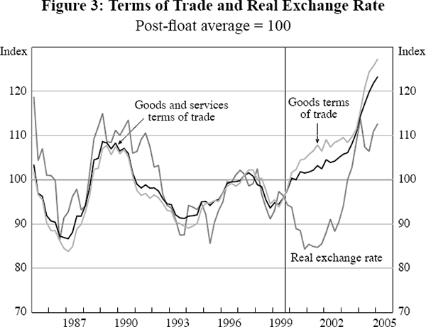
Two issues arise with the continued use of this framework. The first is that, since mid 1999, Australia has experienced a prolonged divergence between the levels of its trade-weighted real exchange rate and terms of trade. From mid 1999 until late 2001 the former underwent a substantial downward shift, even as the latter (whether for goods or goods and services) trended upwards. The resultant gap then closed significantly over 2002 and 2003, but did not disappear – and indeed has opened again over the past 18 months. Such a prolonged and substantial divergence had not previously arisen since the floating of the Australian currency in December 1983, and is not accounted for by the real interest differential between Australia and the rest of the world.
Despite this sustained divergence, we are reluctant to abandon any form of long-run relationship between Australia's real exchange rate and terms of trade, given the strength and durability of the relationship for the preceding 15 years (and the narrowing of the divergence since early 2002). We therefore accommodate this prolonged period of divergence through the introduction of a dummy variable.
The second issue concerns the choice of terms of trade series to use in our real exchange rate model. Beechey et al (2000) used the terms of trade for goods and services, but noted a possible problem with endogeneity between changes in this series and in the real exchange rate.
Such endogeneity could arise because changes in the exchange rate are passed through to import prices faster than to export prices (Dwyer, Kent and Pease 1993), resulting in temporary swings in the terms of trade in response to shifts in the exchange rate. A more general possibility relates to the common assumption that Australia is a price-taker in world markets, so that movements in the exchange rate will have no impact on the terms of trade. While plausible for commodities, and for many increasingly commodity-like manufactured goods, this assumption may not be appropriate for all categories of Australia's trade. In particular, it would seem likely that Australia's services terms of trade is significantly affected by movements in the exchange rate, reflecting the tendency for many service exports to be priced according to domestic considerations.
To overcome this potential endogeneity problem, we use the terms of trade for goods, rather than goods and services, in the model's real exchange rate equation.[12] Accordingly, the current specification of this equation is
where: rer denotes the real exchange rate; tot is the goods terms of trade; rf denotes the foreign real interest rate (proxied by a GDP-weighted average of real short-term policy rates in the G3 economies); pcom is the RBA index of commodity prices in foreign currency terms; sUS is a de-trended real share accumulation index for the US; and r is the domestic real cash rate (defined earlier). Drer denotes the dummy variable included to allow for the divergence between the real exchange rate and the terms of trade over the early years of this decade.[13] Table 2 shows coefficient estimates and associated standard errors for this specification, over the sample 1985:Q1 to 2005:Q1.
| Coefficient | Variable | Value | t-statistic |
|---|---|---|---|
| γ1 | Constant | 0.519 | 2.385 |
| γ2 | Equilibrium correction term | −0.324 | −5.540 |
| γ3 | Terms of trade (level) | 0.629 | 4.943 |
| γ4 | Real interest differential | 1.841 | 3.036 |
| γ5 | US de-trended real share index (change) | −0.182 | −3.245 |
| γ6 | Real exchange rate dummy | −0.057 | −4.029 |
| γ7 | Commodity price inflation | 0.607 | 5.921 |
| Summary statistics | Value | ||
| Adjusted R2 | 0.518 | ||
| Standard error of the regression | 0.029 | ||
| Breusch-Godfrey LM test for autocorrelation (p-value): | |||
| First order | 0.313 | ||
| First to fourth order | 0.108 | ||
| White test for heteroskedasticity (p-value) | 0.143 | ||
| Jarque-Bera test for normality of residuals (p-value) | 0.205 | ||
| Notes: The equation is estimated by OLS using quarterly data over the period 1985:Q1–2005:Q1. All levels variables are in logs except for interest rates (which are expressed in unlogged form as decimals). | |||
A significant role continues to be found for the differential between domestic and foreign real interest rates. This is consistent with Australia's real exchange rate adjusting so as to offset potential gains or losses from shifts in real interest rates in Australia relative to the rest of the world (Gruen and Wilkinson 1991). Overall, the estimated long-run semi-elasticity of the real exchange rate with respect to this differential is now around 1.8 – somewhat stronger than the corresponding figure in Beechey et al of around 1.2.
The equation also finds a role for a lagged change in US real share prices, possibly reflecting that periods of above-average growth in US share prices may provide an early indication of shifts in international flows towards ‘safe haven’ currencies (or, in the late 1990s, towards ‘new economy’ investment opportunities and away from so-called ‘old economies’ such as Australia). The sign of the coefficient on this variable is consistent with such a rationale, and its statistical significance is robust to varying the sample to exclude the 1987 stock market crash.[14]
Finally, unlike in Beechey et al (2000), the model now does find a role for the contemporaneous change in commodity prices, in preference to changes in the goods terms of trade. Commodity prices are widely viewed as an important influence on the real exchange rate due to the large share of commodities in Australia's export basket. We find that, with an added 22 quarters of data, the contemporaneous change in commodity prices now outperforms changes in the goods terms of trade as a short-run explanator for Australia's real trade-weighted exchange rate.[15]
2.3 Import Prices
There are two important changes to the way in which we model import prices, relative to Beechey et al (2000). First, while we continue to model an underlying measure of import prices, this measure now covers both goods and services imports, not just goods imports. This change reflects that, as discussed in Sections 2.5 and 2.6, we model consumer prices as a mark-up over a range of input costs, including import prices. These consumer prices will be influenced by the costs of both goods and services imports, rather than those of goods imports alone.
Secondly, both the foreign export price and nominal exchange rate data we use are now computed on a trade-weighted, rather than G7 GDP-weighted, basis. Beechey et al opted to use the latter for the relative ease with which timely export price data are available for G7 countries. However, the former would seem preferable on theoretical grounds – especially given the breakdown following the Asian crisis in the tendency for Australia's G7 GDP-weighted and trade-weighted nominal exchange rates to move closely together.[16]
Turning to the equation itself, numerous studies have modelled Australian import prices using an equilibrium-correction framework (see, for example, Dwyer et al 1993, Beechey et al 2000 and Webber 1999). Under such a framework, (relative) purchasing power parity (PPP) is typically assumed to hold in the long run, so that the level of import prices should move one-for-one with that of foreign export prices, converted to Australian dollars, in steady state.
Empirically, there are two features of the data since 1985 which might appear to be at odds with such a long-run model. The first is the steady downward trend in the quantity (pm − px,f + e) evident in Figure 4. This suggests that, on average, import prices, pm, have risen less rapidly over the past two decades than the behaviour of trade-weighted foreign export prices, px,f, converted to Australian dollars using the trade-weighted nominal exchange rate, e, would have led one to expect. Fitting a linear trend to the data suggests that this discrepancy has averaged around 0.6 percentage points per annum over the period 1985:Q1 to 2005:Q1.
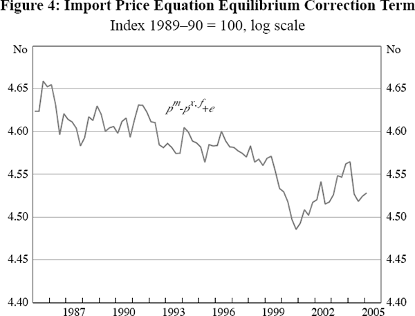
In Beechey et al (2000) a similar but considerably stronger trend discrepancy was reported, which they attributed to their use of G7 GDP-weighted export price and nominal exchange rate measures. The use of such measures, they noted, meant that ‘deviations [from G7 export prices] by non-G7 trading partners will not be captured’, which ‘necessitated the addition of… a time trend to capture the gradual shift in Australia's imports towards lower-priced goods from non-G7 countries (particularly in Asia)’ (p 18). While our move to using trade-weighted foreign export price and nominal exchange rate data appears to have reduced the scale of the trend discrepancy, it has not eliminated it.[17]
One possible explanation for the remaining long-run price growth discrepancy relates to differences regarding the way in which prices of automatic data processing (ADP) equipment are treated statistically in Australia and in other countries. As discussed by Dwyer et al (1993), the Australian Bureau of Statistics (ABS) use a hedonic approach to pricing computer and associated equipment, the effect of which is ‘to equate the dramatic rise in power of computers … with a fall in the unit price of such power’. This approach, however, differs from that adopted by many statistical agencies abroad, and this creates ‘a significant downward bias in Australian import … prices’ relative to the prices recorded for such items by many of the exporters of such equipment to Australia.[18] In any event, whatever the cause of this trend discrepancy, we continue to handle it through the inclusion of a time trend in the long-run component of the model's import price equation.
The second feature of Figure 4 which could seem at odds with a PPP-framework for modelling Australian import prices is the substantial divergence which arose between these prices and foreign export prices (converted to Australian dollars) between 1999 and 2003. During this period, import prices remained persistently below the level which might have been expected given the fall in the exchange rate from 1999 to 2001, together with developments in foreign export prices.
Such a divergence, however, is not necessarily inconsistent with PPP, which relates only to the long-run relationship between import prices and foreign export prices. It may have reflected merely a prolonged reduction in margins by exporters to Australia, anxious to maintain market share in the face of an exchange rate fall which they may not have believed to be a permanent shift. In line with this hypothesis, we choose to view the marked divergence over the period 1999–2003 as a temporary deviation of import prices from equilibrium – albeit a larger and more sustained one than at any other time over the past 20 years.[19]
Overall, the model's import price equation is now specified as follows
where: pm is an index of underlying goods and services import prices (free on board) in Australian dollars; px,f denotes a corresponding trade-weighted index of foreign export prices in foreign currency terms; e denotes the trade-weighted nominal exchange rate; and trendpm denotes a simple time trend. Coefficient estimates and associated standard errors for this specification are shown in Table 3.
| Coefficient | Variable | Value | t-statistic |
|---|---|---|---|
| φ1 | Constant | 0.673 | 2.738 |
| φ2 | Equilibrium correction term | −0.145 | −2.736 |
| φ3 | Time trend | 0.002 | 6.022 |
| φ4 | Foreign export price inflation | 0.813 | 10.757 |
 |
Nominal exchange rate (change) | −0.722 | −30.172 |
 |
Nominal exchange rate (change) | −0.093 | −3.687 |
| Summary statistics | Value | ||
| Adjusted R2 | 0.930 | ||
| Standard error of the regression | 0.008 | ||
| Breusch-Godfrey LM test for autocorrelation (p-value): | |||
| First order | 0.818 | ||
| First to fourth order | 0.306 | ||
| White test for heteroskedasticity (p-value) | 0.127 | ||
| Jarque-Bera test for normality of residuals (p-value) | 0.190 | ||
| Notes: The equation is estimated by OLS using quarterly data over the period 1985:Q1–2005:Q1. All levels variables are expressed in logs. | |||
As in Beechey et al, the equation includes changes in both foreign export prices and the nominal exchange rate as short-run explanators. These variables continue to enter the equation with short lags and sizeable coefficients, so that the adjustment of import prices to shocks in either foreign export prices or the nominal exchange rate remains relatively fast. However, it also remains the case that the coefficients on these terms are such that the joint restrictions required for the equation to exhibit dynamic homogeneity are not accepted by the data.[20]
2.4 Nominal Unit Labour Costs
As in Beechey et al (2000), we use an expectations-augmented Phillips curve to describe the growth of economy-wide unit labour costs (although we now express the equation in terms of quarterly rather than year-ended growth). The output gap is used to capture wage pressures arising from capacity constraints in the economy, while inflation expectations are modelled as a combination of backward-looking (lagged headline inflation and unit labour cost growth) and forward-looking (bond market inflation expectations) components.
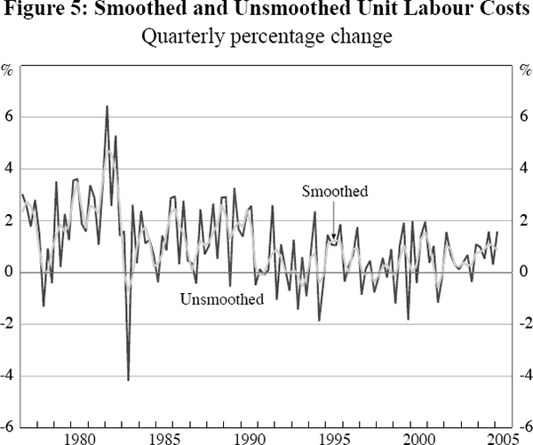
We have, however, made one key change to the treatment of unit labour costs in the model. Rather than working directly with the national accounts-based measure of unit labour costs used in Beechey et al, we choose to model instead a smoothed version of this series.
The reason for this change is that the raw unit labour costs series is highly volatile from quarter to quarter. For example, over the period 1992:Q1 to 2005:Q1 the standard deviation of the quarterly growth rate of this series was 1.04 percentage points, while the average growth rate itself was only 0.42 per cent. By way of comparison, the corresponding figures for (GST-adjusted) headline inflation are 0.31 percentage points and 0.62 per cent, while for (GST-adjusted) median inflation they are 0.19 percentage points and 0.56 per cent.
Of course, the use of a smoothed version of the unit labour costs series would not be justified by the mere presence of such volatility. Indeed, to the extent that such volatility reflects true quarter-to-quarter variability in unit labour cost growth, it would be more appropriate econometrically to leave these fluctuations in the data.
However, it seems likely that some part of this volatility may represent statistical noise, given the indirect way in which unit labour costs data must be inferred from information on aggregate output, hours worked and compensation of employees, and the inevitable difficulties in measuring each of these aggregates precisely. In this event, there would be a cost to leaving such statistical noise in the model's unit labour costs series, whenever attempting to use either the level of this series or its growth rate as an explanator in any of the model's equations. Such noise would result in the ‘errors in variables’ phenomenon of downward bias in the estimated magnitude of relevant coefficients – such as the speed-of-adjustment coefficients (β2 and κ2) on the equilibrium correction components of both the model's headline and median inflation equations (see Sections 2.5 and 2.6 below).
Ultimately, we have chosen to make a smoothed version of unit labour costs the primary measure of such costs in the model, in the hope that this will reduce the extent of noise in the data.[21] We are thus implicitly thinking of this smoothed series as representing a more reliable quarter-to-quarter indicator of the true level of labour costs across the economy, with the raw series representing a ‘noisier’ version of this same series. For comparison, the quarterly changes in both the smoothed and unsmoothed series are shown in Figure 5.
The template Phillips curve for (smoothed) unit labour cost growth we adopt is
where:  represents headline consumer prices adjusted to exclude the impact of the
GST (see Section 2.5 below);
represents headline consumer prices adjusted to exclude the impact of the
GST (see Section 2.5 below);  denotes the deviation
of the quarterly growth rate of our smoothed measure of economy-wide nominal
unit labour costs from
year-ended (GST-adjusted) headline inflation to the prior quarter expressed
in quarterly terms; and
denotes the deviation
of the quarterly growth rate of our smoothed measure of economy-wide nominal
unit labour costs from
year-ended (GST-adjusted) headline inflation to the prior quarter expressed
in quarterly terms; and  denotes the deviation, converted to quarterly
terms, of bond market inflation expectations from year-ended headline inflation.
denotes the deviation, converted to quarterly
terms, of bond market inflation expectations from year-ended headline inflation.
This general specification is then optimised as part of an iterative procedure, outlined in Appendix A, in which potential output is simultaneously estimated. The reason for writing Equation (4) in the form shown is to ensure that, throughout this optimisation procedure, the restriction that the Phillips curve be vertical in the long run is always imposed, regardless of the estimated values of the equation coefficients or of which terms are omitted from the equation. We impose this verticality (or dynamic homogeneity) restriction to ensure that, in steady state, if headline inflation and bond market inflation expectations settle at some common rate then unit labour cost growth will also equilibrate to this same rate. Such a constraint is required to guarantee this, since there is no equilibrium correction term in the unit labour cost equation to tie the long-run level of unit labour costs to that of consumer prices.[22]
It is somewhat involved to test formally whether this verticality restriction is accepted by the data over the whole estimation sample, 1977:Q1 to 2005:Q1.[23] The complication is that the model's potential output data are now constructed concurrently with the estimation of Equation (5). Hence, standard econometric tests of significance are technically rendered invalid by the generated regressor problem (as, strictly speaking, are the OLS-based statistics shown in Table 4).
| Coefficient | Variable | Value | t-statistic |
|---|---|---|---|
 |
Output gap | 0.148 | 7.208 |
 |
Δulc* dev term | 0.614 | 10.306 |
| ρ3 |  terms terms |
−0.145 | −6.529 |
 |
bonddev term | 0.571 | 5.413 |
| Summary statistics | Value | ||
| Adjusted R2 | 0.710 | ||
| Standard error of the regression | 0.005 | ||
| Breusch-Godfrey LM test for autocorrelation (p-value): | |||
| First order | 0.000 | ||
| First to fourth order | 0.000 | ||
| White test for heteroskedasticity (p-value) | 0.856 | ||
| Jarque-Bera test for normality of residuals (p-value) | 0.855 | ||
| Test for vertical long-run Phillips curve (p-value)(a) | 0.485 | ||
|
Notes: The equation is estimated by OLS using quarterly data over the period 1977:Q1–2005:Q1.
All levels variables are in logs except for bond market inflation expectations
(which are expressed in unlogged form as decimals). Although the equation
displays evidence of autocorrelation, the t-statistics
reported are not based on Newey-West corrected standard errors, since any
OLS-derived t-statistics are in any case rendered technically
invalid by the generated regressor problem. If we were to treat the output
gap as exogenous rather than as a generated regressor, however, the Newey-West
correction would not seriously alter the statistical significance of any
of the coefficients reported above. (a) As discussed in greater detail in Appendix B, this test is not strictly correct since the output gap is a generated regressor. However, it is still likely to give a broad indication as to whether or not this restriction is accepted by the data. |
|||
Leaving this issue aside, however – for further discussion of it see Appendix B – the optimisation procedure outlined in Appendix A then yields the following particular specification, coefficient estimates for which are provided in Table 4:
The results in Table 4 suggest that our Phillips curve framework does a reasonable job of explaining the variability in our smoothed, economy-wide measure of unit labour costs over the past 28 years.[24] The coefficient estimates also suggest that employees' inflation expectations are best modelled empirically as a linear combination of lags of (headline) inflation, bond market inflation expectations (converted to quarterly terms) and unit labour costs growth, with respective weights of around 0.25, 0.57 and 0.18.[25]
2.5 Headline Consumer Price Inflation
Following de Brouwer and Ericsson (1998) and Beechey et al (2000) we model headline inflation using an equilibrium correction framework. Under this framework, the level of headline consumer prices is determined, in the long run, by a mark-up over the unit input costs of production. These input costs are assumed to be unit labour costs, import prices and oil prices.
The inclusion of import prices captures the direct cost of imported consumer products, as well as the impact on production costs of those intermediate and capital goods sourced from overseas. We use a tariff-adjusted measure of import prices, pm,trf, to capture the impact of tariffs on final consumer prices. Furthermore, the price of oil, which was considered but not ultimately included by Beechey et al in the equilibrium correction component of their equation, is incorporated here to allow for the fact that the import price index we use is an underlying one which excludes fuel and lubricants.
Unit labour costs are included to capture the cost of domestic labour inputs per unit of output (that is, allowing for labour productivity). Since labour costs associated with the production of exports do not feed into domestic inflation, we need to exclude these from the measure of unit labour costs used in this equation. We therefore use a measure of these costs which, in addition to the smoothing applied as per Section 2.4, is further adjusted for the Balassa-Samuelson effect. This correction accounts for differences in the rate of productivity growth in the traded and non-traded sectors. Details of the precise adjustment adopted, and its implementation in the model, are provided in Appendix C.
One difficulty with adopting an equilibrium correction approach to modelling headline inflation is the lack of a clear cointegrating levels relationship between consumer prices and our three input costs over our preferred sample period from 1992:Q1 to 2005:Q1 – particularly if static homogeneity is imposed on the model. This is the restriction that the long-run elasticities of consumer prices with respect to the three input costs – import prices, oil prices and unit labour costs – should sum to one; or in other words, in terms of the coefficients in Equation (6) below, λm + λo + λu = 1.
We would like to impose such a restriction, to ensure suitable steady-state behaviour (such as the property that, if the levels of import prices, oil prices and unit labour costs were all to double, consumer prices would also double in the long run). However, absent placing an implausibly large weight on oil prices, this restriction would appear to be rejected by the data over the past 13 years – as illustrated by Figure 6.[26]
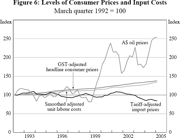
Despite this result, we can ask the following weaker question of the data: if we impose economically plausible values for the long-run elasticities λm, λ0 and λu (see below) which satisfy the static homogeneity constraint, does the resultant mark-up represent a useful explanator of quarterly headline inflation over the period since 1992:Q1?
Interestingly, we find that it does (as is indicated by the statistically significant speed-of-adjustment coefficient, β2, in Table 5 below). Given our strong theoretical preference for static homogeneity to hold in Equation (6), we thus adopt this approach. The elasticities we impose are selected on the basis of both empirical testing and economic plausibility (with reference to factors such as the share of imports as a proportion of GDP and the direct weight accorded to fuel prices in the CPI). These imposed elasticities are 0.2, 0.04 and 0.76 with respect to import prices, oil prices and unit labour costs respectively.[27]
| Coefficient | Variable | Value | t-statistic |
|---|---|---|---|
| β1 | Constant | 0.006 | 7.443 |
| β2 | Equilibrium correction term | −0.078 | −2.837 |
| β3 | GST effect | 0.027 | 8.779 |
| β4 | Output gap | 0.090 | 2.324 |
| β5 | Smoothed, adjusted unit labour cost inflation | 0.223 | 2.672 |
| β6 | Southern Oscillation Index | −0.0001 | −1.459 |
| β7 | Oil price inflation | 0.004 | 1.973 |
| λm | Tariff-adjusted import prices (level) | 0.20 | – |
| λo | Oil prices (level) | 0.04 | – |
| λu | Smoothed, adjusted unit labour costs (level) | 0.76 | – |
| Summary statistics | Value | ||
| Adjusted R2 | 0.720 | ||
| Standard error of the regression | 0.003 | ||
| Breusch-Godfrey LM test for autocorrelation (p-value): | |||
| First order | 0.462 | ||
| First to fourth order | 0.828 | ||
| White test for heteroskedasticity (p-value) | 0.367 | ||
| Jarque-Bera test for normality of residuals (p-value) | 0.412 | ||
| Wald test for equality of coefficients on Δpoil terms (p-value) | 0.758 | ||
| Notes: The equation is estimated by OLS using quarterly data over the period 1992:Q1–2005:Q1. All levels variables are in logs except for the Southern Oscillation Index. | |||
Overall, the model's headline inflation equation is specified as follows
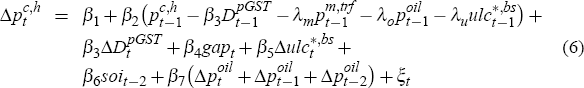
where: pc,h is the headline consumer price index; ulc*,bs is our Balassa-Samuelson-adjusted, smoothed measure of domestic unit labour costs; pm,trf denotes import prices adjusted for tariffs; poil is the Australian dollar price of crude oil; soi is the Southern Oscillation Index; and DpGST is a dummy variable discussed shortly. The speed-of-adjustment parameter β2 captures how much of any disequilibrium between the level of consumer prices and the levels of the three input costs will be removed each quarter, all other things equal. Estimates for this and the equation's other coefficients, together with associated standard errors, are provided in Table 5.
In addition to the equilibrium correction component of Equation (6), other variables used to explain short-run changes in inflation include: changes in (Balassa Samuelson-adjusted) smoothed unit labour costs; changes in oil prices; and the level of the output gap. Consistent with our priors, we find that the coefficients on each of these variables are positive.
A dummy is also included to capture the permanent increase in the price level associated with the introduction of the GST on 1 July 2000. This dummy, DpGST is zero up to and including June quarter 2000 and one thereafter. The coefficient on this dummy, β3, thus represents the model's assessment of the impact of the GST on headline consumer prices, currently estimated to have been 2.7 percentage points. The spike dummy term, β3ΔDpGST, captures the corresponding one-off jump in headline inflation in September quarter 2000 associated with this sustained upward shift in the price level. Note also that the variable pc,h,ex,GST used earlier in Section 2.4 simply denotes the series pc,h − β3DpGST.
Finally, the negative coefficient on the second lag of the Southern Oscillation Index, soi, with a t-statistic of around 1.5, presumably reflects the correlation between negative values of this index and periods of below average rainfall.
Such periods of reduced rainfall typically lead to higher food prices, so boosting headline inflation.
2.6 Underlying Consumer Price Inflation
The model's new underlying inflation equation is also specified as a mark-up model, akin to that for headline inflation. As there, we constrain the equation to satisfy static homogeneity by imposing the same long-run elasticities with respect to input costs as for headline consumer prices: λm = 0.2, λo = 0.04 and λu = 0.76. Our preferred underlying inflation equation is as follows
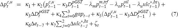
where pc,u denotes an index of underlying (weighted median) consumer prices, and all other variables are as discussed previously. Coefficient estimates and associated standard errors for this equation, over the sample 1992:Q1 to 2005:Q1, are shown in Table 6.[28]
| Coefficient | Variable | Value | t-statistic |
|---|---|---|---|
| κ1 | Constant | 0.006 | 7.814 |
| κ2 | Equilibrium correction term | −0.058 | −3.758 |
| κ3 | GST effect | 0.026 | 16.784 |
| κ4 | Output gap | 0.019 | 4.147 |
| κ5 | Lagged GST-adjusted underlying inflation | −0.274 | −2.190 |
| κ6 | Nominal exchange rate (change) | −0.015 | −2.434 |
| κ7 | Smoothed, adjusted unit labour cost inflation | 0.062 | 3.304 |
| λm | Tariff-adjusted import prices (level) | 0.20 | – |
| λo | Oil prices (level) | 0.04 | – |
| λu | Smoothed, adjusted unit labour costs (level) | 0.76 | – |
| Summary statistics | Value | ||
| Adjusted R2 | 0.893 | ||
| Standard error of the regression | 0.001 | ||
| Breusch-Godfrey LM test for autocorrelation (p-value): | |||
| First order | 0.347 | ||
| First to fourth order | 0.240 | ||
| White test for heteroskedasticity (p-value) | 0.541 | ||
| Jarque-Bera test for normality of residuals (p-value) | 0.266 | ||
| Notes: The equation is estimated by OLS using quarterly data over the period 1992:Q1–2005:Q1. All levels variables are expressed in logs. Note that the statistics reported here are rendered technically invalid by the generated regressor problem, since this equation is used as one of the conditioning equations for estimation of the output gap. However, this is unlikely to be causing any of the coefficient estimates or t-statistics above to be seriously misrepresented (see Appendix B for further details). | |||
Comparing the short-run dynamics of the model's headline and underlying inflation equations, both contain suitable dummies for the impact of the GST on consumer prices in September quarter 2000 – with the estimated GST effect on underlying prices of 2.6 percentage points very similar to that for headline prices. Both equations also contain output gap and unit labour cost inflation terms, albeit with different lag structures. However, unlike for headline inflation, there is no role for lagged changes in Australian dollar oil prices in the underlying inflation equation. This is consistent with such oil prices being distinguished by large quarterly swings. When such swings occur they tend to lie in one or other tail of that quarter's distribution of price changes for the roughly one hundred goods and services categories which make up Australia's CPI basket. Hence, they would not be expected to affect weighted median inflation in that quarter.[29]
In a similar vein, no role is found for lags of the Southern Oscillation Index in the underlying inflation equation. This accords with our earlier rationale for the presence of such a term in the headline equation. Occasional drought-related surges or collapses in food prices also tend to lie in the tails of the relevant quarter's consumer price change distributions, and so directly affect headline but not weighted median inflation. Finally, the underlying inflation equation also includes: the first lag of (GST-adjusted) underlying inflation itself; and a long lag of the change in the nominal exchange rate, presumably supplementing the role of the equation's equilibrium correction term in capturing the gradual pass-through of exchange rate shifts into consumer prices via import prices.[30]
Footnotes
Note that, throughout the remainder of the paper, levels variables such as actual and potential output, consumer prices, import prices and unit labour costs are expressed in log terms, unless otherwise stated. Hence, period-on-period changes in these variables may be interpreted, to a very good approximation, as percentage growth rates expressed as decimals. The principal exception is interest rates, which are not converted to logs, but are also expressed as decimals for consistency. [8]
This dummy variable is chosen to reflect observed shifts in the timing of activity associated with the introduction of the new tax system. It is set equal to one in the December quarter 1999 and negative one in the December quarter 2000, with the majority of changes to the tax system having taken formal effect on 1 July 2000. [9]
The contemporaneous change in the US gap provides a better fit than either current or lagged levels of this gap. Note that US potential output growth in the model is fairly stable over time. This variable is thus little different (up to a constant) from the contemporaneous growth rate of US real output. [10]
Alternatively, Australian share prices may simply be forward-looking, and so provide an early indication of the likely strength of future activity, without necessarily playing any causal role. [11]
An alternative would be to control for possible endogeneity by using instrumental variables estimation. Beechey et al found that this yielded little evidence of simultaneity bias, and did not reduce the extent of short-run overshooting of the exchange rate in response to terms of trade shocks. We find that use of the goods terms of trade does reduce the short-run responsiveness of the exchange rate to such shocks, compared with that implied by using the goods and services terms of trade, but that the difference is not large. [12]
The value of this dummy increases linearly from 0 to 1 over 1999–2000, remains at 1 over 2000–01 and 2001–02, and then decreases linearly to 0 again over 2002–03. Of course, the need for such a dummy in the recent past suggests that more than usual caution would be called for if including this equation as part of generating any forecasts using the model – at least until it becomes clearer whether or not the previous levels relationship between Australia's real exchange rate and terms of trade has indeed reasserted itself. An obvious alternative, for purposes of generating such forecasts, would be to ‘turn the equation off’ temporarily and instead impose an exogenous assumption for either the real or nominal exchange rate. [13]
We experimented with using instead, either in levels or in changes, lags of the difference between de-trended real share accumulation indices for the US and Australia. Despite such terms being theoretically preferable, the equation displays a strong empirical preference for use of the US index alone. [14]
Indeed, we find that the use of  in place of tott−1 in the equilibrium correction
component of the model would produce a further improvement in the equation's
goodness-of-fit. However, this improvement is slight. We therefore opt not
to incorporate this change in light of the difficulty of settling on a suitable
steady-state assumption for the level of commodity prices, a nominal variable,
relative to doing so for the goods terms of trade.
[15]
in place of tott−1 in the equilibrium correction
component of the model would produce a further improvement in the equation's
goodness-of-fit. However, this improvement is slight. We therefore opt not
to incorporate this change in light of the difficulty of settling on a suitable
steady-state assumption for the level of commodity prices, a nominal variable,
relative to doing so for the goods terms of trade.
[15]
In the aftermath of the Asian crisis the value of the Australian dollar fell much more sharply in G7 GDP-weighted terms than on a trade-weighted basis, reflecting the even larger falls in the currencies of many of Australia's Asian trading partners. [16]
Theoretically, a further shift to using import- rather than trade-weighted foreign export price and nominal exchange rate data would seem appealing in this equation. However, we find that doing so does not help to reduce the remaining discrepancy. Hence, in the interests of parsimony, we continue to use a single trade-weighted nominal exchange rate measure throughout the model. [17]
Consistent with this hypothesis, if we replace our preferred import price index with one which excludes ADP equipment prices we find that the quantity (pm ex ADP − px,f + e), rather than trending downwards over time, gradually drifts upwards. This reflects that ADP equipment prices, which have consistently exhibited weak or negative price growth over the past 20 years, are thereby excluded from Australia's import prices but not from foreign export prices. [18]
The unusual character of this divergence could alternatively be handled through the introduction of a suitable dummy variable – akin to Beechey et al's use of a dummy in their import price equation to ‘capture extra price-undercutting by Asian exporters following the Asian crisis’. [19]
These restrictions are that φ4 = 1 and  (see Beechey
et al for a detailed explanation). For a brief discussion of the implications
of this rejection, see Section 3.2.
[20]
(see Beechey
et al for a detailed explanation). For a brief discussion of the implications
of this rejection, see Section 3.2.
[20]
Specifically, we use a 5-term Henderson moving average to generate this smoothed series. This choice is motivated by our desire to apply a ‘light touch’ in the smoothing process, softening rather than fully overriding the quarter-to-quarter fluctuations in the unit labour costs data. [21]
As in Beechey et al (2000), we were unable to find a statistically significant
role for such an equilibrium correction term, 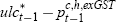 , in Equation (4).
[22]
, in Equation (4).
[22]
For their analogous Phillips curve, Beechey et al were unable to impose such a restriction over their whole sample, 1985:Q1 to 1999:Q3. They were thus forced to resort to imposing the restriction only from 1996:Q1 onwards – on which it was easily accepted by the data. [23]
As a check on the appropriateness of our use of a smoothed version of unit labour costs, it is interesting to re-estimate Equation (5) with unsmoothed quarterly unit labour costs as the dependent variable. Since our appeal to the ‘errors in variables’ phenomenon strictly only justifies our using a smoothed measure of unit labour costs on the right-hand side of Equation (5), we would hope that this would leave the equation's coefficients largely unchanged (notwithstanding the reduction in the equation's adjusted R2). Happily, this is indeed what we find, which supports our decision to use only our smoothed measure of unit labour costs throughout Equation (5) – as well as in Equations (6) and (7) below – on the grounds of parsimony. [24]
These figures represent the combined coefficients on  terms, on
  terms and on
  terms when the relevant right-hand side variables in Equation (5) are unravelled
and re-grouped.
[25]
terms when the relevant right-hand side variables in Equation (5) are unravelled
and re-grouped.
[25]
In part, the problem may stem from our choice of sample period. This starts after the downward shift in inflation associated with the early 1990s recession, lest the inflation process itself was different in the high inflation era of the 1970s and 1980s (see Dwyer and Leong 2001 for a discussion of this issue). Since that time, however, the Australian economy has experienced an abnormally long period of expansion (barring a single quarter of negative growth in December quarter 2000). As a result, our sample does not yet include even a single full business cycle, the period over which the mark-up of consumer prices over input costs would typically be expected to fluctuate. That said, other more fundamental issues also appear to be playing a role. In particular, alternative consumer price measures which might be natural candidates for a mark-up model – such as the implicit price deflator for private consumption in the national accounts – have exhibited markedly different average growth rates over our sample period. This illustrates the difficulty of trying to fit a mark-up model based on our standard set of input costs, with static homogeneity imposed, to any one of these alternative consumer price series. [26]
It is interesting to note that Heath, Roberts and Bulman (2004) report a long-run elasticity of consumer prices with respect to import prices of 0.17, for a similar mark-up model of inflation, over the sample 1990:Q1 to 2004:Q1 (see Table 6, p 191). In obtaining this estimate, however, they did not impose a static homogeneity constraint, and the import price measure they used excluded ADP equipment prices. [27]
As with headline prices, the series pc,u,exGST is then defined simply to be pc,u − κ3DpGST. [28]
The slower second-round impact of sustained shifts in oil prices on median prices, through changes in general production and distribution costs, is still captured through the presence of the oil price level in the equation's equilibrium correction term. [29]
Surprisingly, the seventh lag of the change in the exchange rate performs marginally better in explaining median inflation than a similar direct lag of import price inflation. The negative coefficient on this term indicates that an appreciation of the exchange rate reduces underlying inflation with a long lag, beyond its impact through the model's equilibrium correction term. [30]