RDP 9510: Modelling Inflation in Australia 5. A Single Equation Model of Inflation

The following three sections present estimation results for a single-equation error correction model of inflation. To start, analytical relationships between autoregressive distributed lag models (ADLs), error correction models (ECMs), and the long-run solution (2) are discussed (Section 5.1). An estimated long-run solution is obtained from an autoregressive distributed lag of the CPI on unit labour costs, import prices, petrol prices, and an output gap; and a parsimonious ECM is derived from that autoregressive distributed lag (Section 5.2). The ECM has sensible economic and statistical properties (Section 6), it encompasses existing models (Section 7.1), and it may be useful in forecasting (Section 7.2). Readers familiar with ECMs and autoregressive distributed lags may skip directly to Section 5.2.

5.1 Autoregressive Distributed Lags, ECMs, and Long-Run Solutions

With the choice of variables and lag length in the vector autoregression above, a fourth-order autoregressive distributed lag model in p, ulc, ip, and pet is a natural starting point for single equation modelling. This regression is modified in two ways. First, the output gap y^res is included to reflect how the mark-up μ – 1 may vary over the cycle. Second, a dummy D is included for an increase in indirect taxes in December 1978.^[7] Thus, the fourth-order ADL of the underlying CPI is:

where u_t is the error term. As with the cointegration analysis, a constant term and seasonal dummies are included: S_it denotes the centered (zero mean) seasonal dummy for the ith quarter.

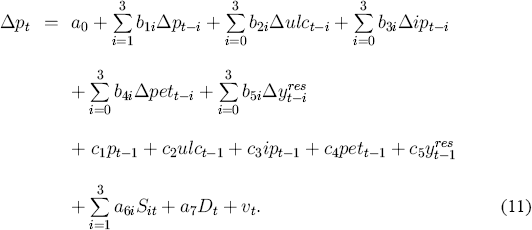
Equation (10) may be reparameterized without loss of generality as an unrestricted ECM by adding and subtracting lags of the variables:

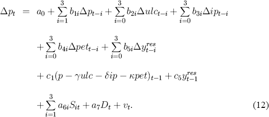
With minor algebraic manipulation, equation (11) may be rewritten so as to incorporate the long-run solution (2) directly.

Specifically, c₁ (with c₁ < 0 for dynamic stability) is the feedback coefficient for the measure of disequilibrium,

which is the empirical mark-up in the previous period. The coefficients γ, δ, and κ, are −c₂/c₁, −c₃/c₁, and −c₄/c₁, which are the long-run elasticities in (2).

Some straightforward algebraic manipulation of (11) obtains various equilibrium solutions, including the solution (2). Extensive discussions of the relationship between the ECM and its long-run solutions appear in Davidson, Hendry, Srba and Yeo (1978), Hendry, Pagan and Sargan (1984), and Hendry (1995). Under a non-stochastic static-state equilibrium, the output gap, all growth rates, and the error term u_t are zero in (11); time subscripts are dropped; and the seasonals and dummy can be ignored. That leaves (11) with the constant a₀ and the levels p, ulc, ip, and pet. Moving p to the left-hand side and renormalizing, (11) solves for (2):

The superscript s in p^s indicates that (14) is the static equilibrium. The constant term –a₀/c₁ in (14) is equivalent to ln(μ) in (2), where the latter is the logarithmic approximation to the mark-up μ – 1. Thus, the error correction model (11) solves for the long-run solution (2) when evaluated under the non-stochastic static-state assumptions associated with (2).

Equation (14) is the static equilibrium of the ECM (11), where static means assuming that all prices are constant. More generally, (11) might be evaluated under various steady-state (rather than static-state) assumptions. Under one such set of assumptions, all prices grow at some constant rate g (Δp = Δulc = Δip = Δpet = g) and the output gap y^res is constant but possibly nonzero. That is, a nonzero inflation rate and a nonzero output gap are two simple aspects of a dynamic equilibrium.^[8] Solving (11) for p in a similar manner to that done for (14), the resulting dynamic equilibrium price level p^d is:

where ø is a complicated function of {b_ji,j = 1,...,4} and c₁. Equation (15) generalizes (14) for nonzero price growth rates and a nonzero output gap. In particular, the logarithmic approximation to the mark-up is – (a₀/c₁) – øg – (c₅/c₁)y^res rather than just –(a₀/c₁): the inflation rate and the output gap influence the mark-up, and so influence the level of the CPI relative to other prices. This formulation captures a way in which the mark-up might vary over the cycle.

For each of (14) and (15), a time series of disequilibria can be constructed by subtracting the right-hand side of the respective equation from p, evaluating all variables at observed values. These disequilibrium measures are denoted u^s and u^d respectively.

This paper presents estimates of the coefficients in (14) under different assumptions. In the VAR framework of Section 4.2, equations (6), (7), and (8) respectively assume nothing, long-run price homogeneity, and long-run price homogeneity and weak exogeneity. In the single equation framework of Sections 5.2 and 6.1 below, (16) and (18) respectively assume weak exogeneity only, and weak exogeneity, long-run price homogeneity, and a simplified lag structure. Comparison of estimates across these various equations indirectly assesses the associated assumptions themselves. Section 6.1 also reports the dynamic solution (15) and compares the static and dynamic equilibrium prices with actual prices, both directly and through the corresponding disequilibrium measures u^s and u^d.

Equation (12) generalizes the conventional partial adjustment model by allowing separate reaction speeds to the different determinants of the CPI, reflecting potentially different costs of adjustment and of disequilibrium. Through the error correction term, (12) allows discrepancies between the log-level of the CPI and its determinants to affect future inflation, thus keeping the level of the CPI “in line” with its determinants in the long run. Economically, (12) is related to Ss-type models, with short-run factors determining CPI movements within a given price environment and longer-run factors determining the general level of prices. In particular, short-run factors affect the mark-up itself. For further details, see Nickell (1985) for an optimizing framework that results in an error correction model, and Smith (1986) for the ECM's relation to Ss inventory models, albeit in the context of money demand.

The ECM (12) is a remarkably general model. In particular, it contains both static levels models and pure difference models of inflation as special (and testable) cases. The ECM's relation to models in levels follows from the equivalence of (12) with the ADL in (10), and restricting the ADL such that all a_ji are zero for j = 1,..., 5 and i > 0. The ECM's relation to models in differences follows directly from (12) with c₁ (and possibly c₅) set to zero. Thus, models in differences contain no information about the long run, i.e., on the levels. As is readily apparent from the empirical ECM (17) developed in Section 5.2, neither static models nor models in differences alone are empirically satisfactory. Section 7.1 further discusses these issues in the context of encompassing.

Ostensibly, equation (12) explains inflation. It also determines the price level through its relationship with (10), provided c₁ ≠ 0. For detailed discussion on the algebra of ECMs, see Hendry, Pagan and Sargan (1984), Ericsson, Campos and Tran (1990), and Hendry (1995).

5.2 General to Specific Modelling

This subsection simplifies the fourth-order ADL to a parsimonious ECM. Sections 6 and 7 examine the estimated model's economic and statistical properties in greater detail.

Most of the individual coefficients in the fourth-order ADL (10) are imprecisely estimated and are of little interest in themselves. However, the long-run solution of the ADL is of interest, and its coefficients are well-determined:

where estimated standard errors are in parentheses (·). Equation (16) corresponds to (2) and (14). The estimates in (16) are very close to those obtained by Johansen's analysis of the VAR. Simplification of the fourth-order ADL to a first-order ADL is statistically acceptable, and achieves a virtually identical long-run solution with somewhat smaller standard errors, paralleling the system result that only first lags matter.

When the fourth-order ADL is transformed to the unrestricted ECM representation (11), many of the coefficients are both economically and statistically insignificant; see Table A2 in Appendix 2. For instance, no lags (other than lagged log-levels) appear important. These and other restrictions described in Appendix 2 provide a natural path for the simplification of (11) to the following highly parsimonious, economically interpretable, and statistically acceptable ECM.

T = 65 [1977(3)–1993(3)]	R2 = 0.87	= 0.251%
AR : F(5, 50) = 0.59	dw = 1.98	ARCH : F(4, 47) = 0.85
Normality : χ2(2) = 2.24	RESET : F(1, 54) = 0.22
Hetero : F(14,40) = 0.99	Inn : F(19,36) = 0.66
LMp : F(1,54) = 0.09.

In (17), just three economic variables affect CPI inflation: the current change in petrol prices, the previous quarter's output gap, and the previous quarter's mark-up. These variables are all statistically significant, particularly the latter two. The output gap and the change in petrol prices have positive effects; and the mark-up has a negative effect, as required for dynamic stability of the equation. Indirect taxes (through D_t) and seasonality also affect inflation. The coefficients in (17) are consistent with the mark-up model (2), where the mark-up itself varies with the output gap. Section 6 considers the dynamic and long-run implications of the variables in (17) at greater length, showing how to obtain those implications from the analytics of Section 5.1.

Equation (17) lists diagnostic statistics for testing against various alternative hypotheses: residual autocorrelation (AR and dw), autoregressive conditional heteroscedasticity (ARCH), skewness and excess kurtosis (Normality), RESET (RESET), heteroscedasticity (Hetero), and non-innovation errors relative to the fourth-order ADL (Inn).^[9] The null distribution is designated by χ²(·) or F(·,·), the degrees of freedom fill the parentheses, and (for AR and ARCH) the lag order is the first degree of freedom. Statistically, the ECM appears well-specified, with no rejections from the tests available. Also, the imposed restriction of long-run price homogeneity is not rejected by the appropriate Lagrange multiplier statistic (LM_p).

For convenience, the ECM (17) will be called the preferred equation. Appendix 3 develops an alternative ECM, which contains an additional term for the dynamic effects of the business cycle on inflation.

Footnotes

While the output gap and the dummy D_t may capture economically and statistically important behaviour in prices, their effects are viewed as short run and so are not included in the cointegration analysis above. If included, the cointegration results are virtually unchanged. [7]

Other dynamic equilibria exist, e.g., ones with nonzero growth rates in real prices such that the error correction in (12) is constant. However, the solution in (15) is the simplest of the dynamic equilbrium paths; and it has a certain economic appeal in that all real prices are assumed constant. [8]

For references on the test statistics, see Durbin and Watson (1950, 1951), Box and Pierce (1970), Godfrey (1978), and Harvey (1981, p. 173); Engle (1982); Jarque and Bera (1980) and Doornik and Hansen (1994); Ramsey (1969); White (1980, p. 825) and Nicholls and Pagan (1983); and Hendry (1995) respectively. [9]