RDP 9510: Modelling Inflation in Australia Appendix 3: An Alternative Model of the CPI

This appendix discusses the measure of the output gap y^res, and then develops an alternative model to (17) that captures dynamic effects of the output gap on inflation.

In (17) and in (A1) below, the output gap is incorporated explicitly as y^res. The empirical results are little affected if y and a trend enter freely. For instance, if (17) is estimated unrestrictedly, the coefficient on the trend (−0.000515) is approximately equal to minus the coefficient on y_t–1 (0.0769) multiplied by the regression coefficient of y on a trend (e.g., 0.00694 from equation (5)). The role of the unrestricted trend is solely to detrend y_t–1, and the regression coefficient on y_t–1 is interpretable as the effect on inflation of a deviation of y_t–1 from its trend. Also, while potential output is estimated in (5) by a linear time trend, the results are not sensitive to its specification as such or as (e.g.) the trend generated by a Hodrick-Prescott filter of y.

Conceptually, y^res is more a measure of a demand gap than of an output gap because Y is private final demand rather than (e.g.) GDP. Constructed measures of a gap from the two variables are very similar, and the choice of GDP rather than private final demand makes little difference to the estimated equations. Because private final demand is commonly used in Australia for assessing the state of the domestic business cycle, the former was selected to calculate y^res, rather than GDP. The phrase “output gap” is then a convenient but slightly misleading label for y^res.

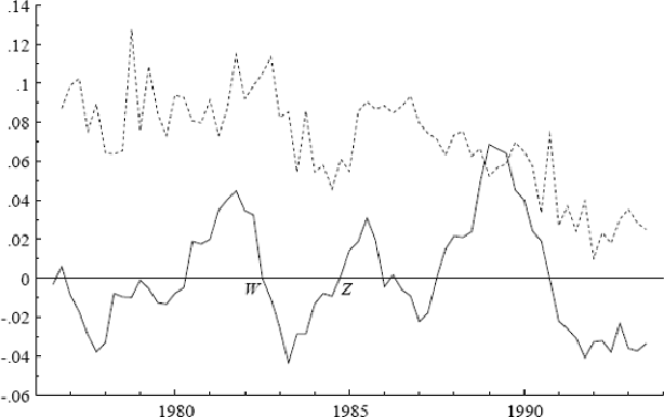
In the ECM (17), the output gap y^res is included to capture the effect on inflation of deviations of output from potential. The effect of the business cycle on inflation, however, may also depend upon how strong recent growth in the economy has been. To illustrate, consider the two points W and Z in Figure A4, which plots quarterly inflation at annual rates and the output gap y^res. The values of actual y relative to trend are equal at W and Z, even while the points W and Z are at different stages of the cycle. At W, y^res has come off its peak and is falling but inflationary pressures may still remain. At Z, y^res has recovered from its trough but inflationary pressures may be slow to resurface. In short, inflationary pressures may tend to lag the cycle, in which case the change in the output gap Δy^res as well as its level y^res may contain information about inflation.

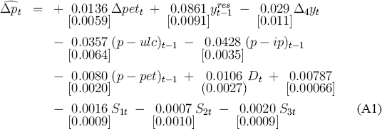
This additional effect of the cycle may be incorporated into the ECM (17) by adding the growth rate of private final demand, noting that Δy and Δy^res differ by only a constant. The results are presented below in (A1), where the growth rate in private final demand is annual (Δ_4yt). This variable is statistically significant, with a negative coefficient as expected.

The specification in (A1) explains the data somewhat better than the ECM (17), but at the expense of slightly greater complexity.

Some explanation is required to account for the performance of (17) in spite of its omission of Δ_4yt. Four quarterly growth rates comprise Δ_4yt: Δ_yt, Δ_yt−1, Δ_yt−2, and Δ_yt−3. Only one quarterly growth rate (Δ_yt) is statistically significant if added to (17), and jointly these growth rates are statistically insignificant. However, the growth rates are statistically significant when their coefficients are imposed to be equal. The sequential reduction in Appendix 2 failed to detect the presence of Δ_4yt because each of the first three reductions dropped the longest lag on all variables, rather than (e.g.) focusing on the lags of a given variable, one variable at a time. Equally, Δ_4yt could only marginally improve the fit of (17), given the ease with which the sequential reduction in Appendix 2 excluded it.

The model in (17) is the focus of the paper because it is slightly more parsimonious than (A1) and with little loss of fit. Both models have very similar statistical properties and economic interpretations. While the point estimates of the long-run elasticities from (A1) are different from those obtained earlier, they are not statistically significantly so. For forecasting in the contemporary economic environment, the effect of the higher import price coefficient in (A1) would be offset by the lower inflationary pressure associated with recovery (through the term Δ_4yt).