RDP 9510: Modelling Inflation in Australia 6. The Model's Properties

This section considers the economic interpretation and statistical properties of the ECM in (17). Sections 6.1 and 6.2 focus on the long-run and dynamic properties of the model, Section 6.3 demonstrates the model's empirical constancy, and Section 6.4 offers a few caveats.

6.1 Long-Run Properties of the Model

The long-run properties of an error correction model can be characterized by its static and dynamic solutions (p^s and p^d), and by the implied dise-quilibria from those solutions (u^s and u^d). This subsection analyzes those solutions and associated disequilibria, both numerically and graphically.

Equation (17) embeds the mark-up model (2) in its static long-run solution p^s, which is:

corresponding to (14). The dynamic equilibrium solution p^d is:

as derived from (15). Long-run homogeneity is statistically acceptable and is imposed in (18) and (19). The estimates of the long-run solution in (18) from the ECM are numerically close to the system estimates of the cointegrating vector in (6), (7), and (8), and to the single equation estimates in (16) from the unrestricted ADL. This robustness of results provides some indirect evidence in favour of the assumptions imbedded in the final ECM relative to the unrestricted VAR. The tests above of long-run homogeneity, weak exogeneity, and innovation errors provide the direct evidence.

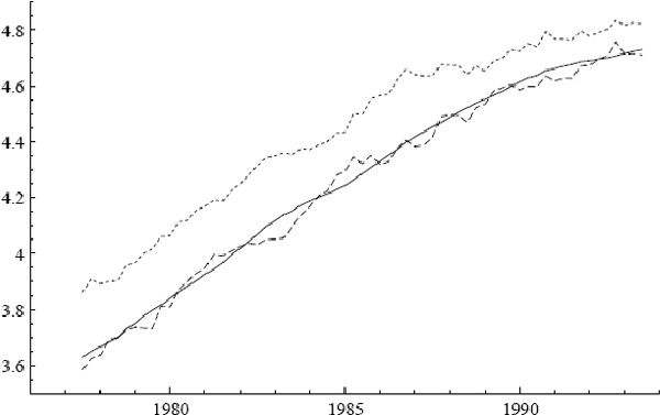
Consumer prices, their static equilibrium, and their dynamic equilibrium are shown in Figure 10. To calculate p^s and p^d for the figure, current-dated variables are used on the right-hand side of (18) and (19). Further, g must be specified for (19); and the average is used so as to smooth the relatively erratic inflation series. Seasonal dummies as well as the constant term are included in calculating both p^s and p^d. Actual prices and the dynamic equilibrium path are quite similar: deviations between them (u^d) are typically only a few per cent, with those deviations lasting a year or two at a time; see Figure 11. Recently, actual prices have been particularly close to the dynamic equilibrium path. By comparison, the static equilibrium path consistently lies above actual prices, often by 20% to 30%. This discrepancy (u^s) primarily reflects omission of the term –øg from the calculation of p^s in (14). The estimate of –ø in (19) is large and negative (−11.1), and the quarterly inflation rate often is 2% to 3%, implying discrepancies of the magnitude observed and contrasting with the zero inflation rate assumed in solving for p^s.

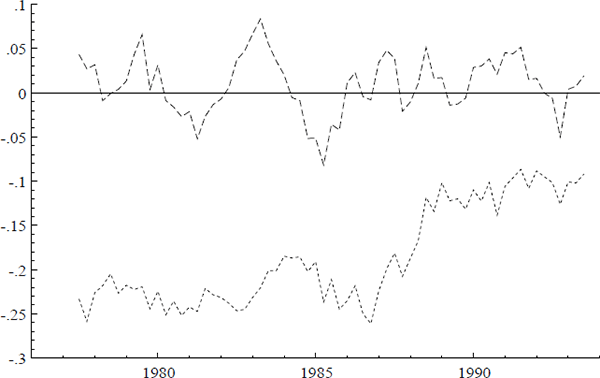
The importance of the growth rate g in the dynamic equilibrium solution has different interpretations. Most straightforwardly, ln(μ), the mark-up from (2), depends negatively on g. As g declines in the late 1980s and the early 1990s, the mark-up increases, as seen from the plot of p – p^s in Figure 11. More subtly, p, ulc, ip, and pet might be I(2), cointegrating as in (2) to form an I(1) linear combination, which itself could cointegrate with the inflation rate (I(1) here by assumption) to form an I(0) combination. The dynamic equilibrium (19) would then be that I(0) combination. In principle, p, ulc, ip, and pet might be I(2), although a nonstationary mark-up is economically unappealing. For Australia with this data, p, ulc, ip, and pet appear to be I(1) empirically. The ADF statistics and estimated coefficients in Table 1 and the multivariate stationarity tests in Table 2 support that these variables are I(1). Also, Johansen's (1992c) analysis implies that variables are at most I(1) if, as in the VAR considered above, their vector autoregression is first order with a single cointegrating vector, weak exogeneity for that cointegrating vector, and a nonzero cointegrating coefficient on the endogenous variable. As an intermediate alternative, p, ulc, ip, and pet might be I(1) and cointegrated, but with their mean growth rates shifting down in the latter part of the sample. If the mark-up depends upon g, then the mark-up might appear nonstationary because of that shift in g; see Campos, Ericsson and Hendry (1996).

Both disequilibrium measures u^s and u^d are stationary series in that they correspond to the observed cointegrating vector. That said, both series appear to be nonstationary from the augmented Dickey-Fuller statistics in Table 1. This seeming contradiction is resolved by the higher power of the Johansen procedure relative to ADF statistics for detecting the stationarity of multivariate relationships. Equally, a univariate procedure such as the ADF statistic is at an inherent disadvantage when used to evaluate multivariate hypotheses such as cointegration.

The long-run coefficient estimates are plausible and sensible. Numerically, the coefficient on unit labour costs is the largest and that on fuel prices the smallest. This accords with conventional wisdom. The coefficient on import prices is perhaps a little more controversial, and is not statistically different from that on unit labour costs. Specifically, the coefficient is higher than 0.2 – 0.3, which is a range quoted by some commentators and which is similar to the import propensity for all goods and services (about 0.2). The estimated elasticity bears on the potential inflationary impact of recent exchange rate depreciations. The Australian dollar depreciated by over 10% between March and August in 1992 and by 5% in May 1993. The ECM (17) indicates that the CPI eventually rises by 0.44% for every 1% permanent increase in import prices. The import elasticity in (17) may depend on the definitions of the right-hand side variables selected, and other definitions and specifications may yield different results. Still, this result is robust across the specifications considered herein.

Several factors may account for the higher estimated import price coefficient in (17). First, many pre-existing models of the CPI were in growth rates only, so the imputed long-run elasticities were actually short-run rather than long-run. For example, estimating equation (11) as a distributed lag model with six lags but without the error correction term yields a solved import price coefficient of about 0.2. From Section 6.2 below, 0.2 is approximately the six-period cumulated response implied by (17). Second, the appropriate benchmark for the import price effect is, at a minimum, the share of importables rather than the share of imports, with the former being larger than the latter. Third, the market for exportables may be important. If the price of exportables sold in the domestic market is set at the world price (which is assumed to be given to exporters), then this creates an additional channel by which a depreciation will be inflationary. Since movements in import prices are dominated by movements in the exchange rate, an effect from the price of exportables will be picked up by the import price series. Fourth, if domestic producers and retailers price strategically or attempt to maintain some relativity to import prices, then the import price coefficient will be higher than the importables propensity. Fifth, as mentioned above, many previous models of Australian CPI were estimated in differences only, with smaller estimated “long-run” elasticities for imports. To the extent that comparisons are made, it seems plausible that those earlier results are biased downward from using differences only.

Finally, the modelled CPI is the underlying CPI, not headline CPI. The underlying CPI accounts for approximately 80% of the headline CPI. So, using equation (17), the long-run effect of a change in import prices on headline CPI is about 0.36 (or about 0.38 if the share of petrol is excluded), assuming that import prices do not influence the price of items excluded from the underlying CPI. It is also worth noting that the numbers in (17) are point estimates: plus-or-minus two standard errors on the estimated import price elasticity yields a confidence interval of 0.34 to 0.54.

6.2 Dynamic Properties of the Model

Equation (17) has several implications for lags and lag distributions and for the economic interpretation of the error correction term. First, the CPI adjusts slowly to shocks, even though lag lengths in (17) are short. Representation of the ECM as an ADL helps clarify this apparent disparity, as does solving for the implied lag distributions of the estimated ECM. Second, the error correction term in (17) is interpretable as capturing feed-backs from the domestic labour market, the foreign goods market, and the energy market.

In (17), adjustment to disequilibrium is very gradual, even though no lags beyond the first are necessary in that equation (see Appendix 2). The explanation follows from the small coefficient on the error correction term (−0.0891) and small or zero coefficients on contemporaneous variables. When rewritten as the autoregressive distributed lag representation (10), equation (17) becomes:

where the constant, seasonals, and dummy D are omitted for simplicity of exposition. The small ECM coefficient in (17) implies a large coefficient (0.9109) on the lagged dependent variable p_t–1 in (20), generating long solved distributed lags of unit labour costs, import prices, energy prices, and the output gap.

For example, suppose import prices increase permanently by 10% in a given quarter. Current-dated import prices do not appear in (20), so the contemporaneous response of the CPI is zero. One quarter later, the CPI increases by 0.394%, noting that the coefficient on ip_t–1 in (20) is 0.0394 (equivalently, (−0.0891).(−0.443) from (17)). In each succeeding quarter, the disequilibrium is reduced by progressively smaller increments until the full 4.43% increase in the CPI is achieved, corresponding to the long-run elasticity of 0.443 for import prices. This adjustment is a drawn-out process, with just half of the adjustment completed after two years, and only three-quarters of the adjustment completed after four years.^[10]

Thus, the model (17) incorporates the appealing idea that permanent increases in costs increase the CPI in the long run whereas temporary increases in costs have small short-run effects. This is especially sensible here since unit labour costs, import prices, and petrol prices can be very volatile on a quarter-to-quarter basis. For import prices in particular, the lag structure implies that the path of the exchange rate in the few years before a depreciation mediates the proximate inflationary effect of that depreciation. The ostensible deflationary effect of the recent appreciation in the exchange rate should be viewed similarly.

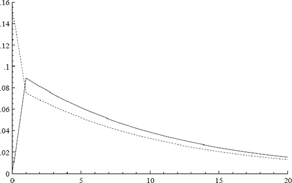
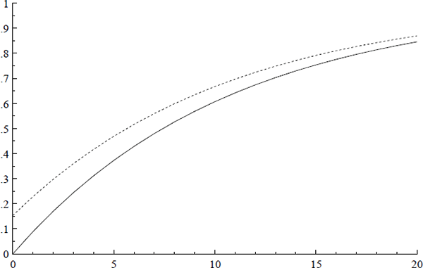
Explicit lag distributions and functions thereof are easily calculated numerically. Figure 12 plots the derived normalized lag distributions for ulc_t, ip_t, pet_t, and from equation (17).^[11] Their median lags are 7, 7, 6, and 7 quarters respectively; and their mean lags are all somewhat greater than two years. Figure 13 plots the normalized cumulative lag distributions, from which the median lags are derived. Figures 12 and 13 also represent the responses of the CPI to suitably normalized temporary and permanent changes in the corresponding variables, thereby providing graphical assessment of the numerical calculations in the previous paragraphs. The relatively small error correction coefficient and contemporaneous short-run elasticities imply substantial smoothing in the price process and major differences between short- and long-run elasticities for a given variable.

Some previous models of the Australian CPI are in differences only and require substantially longer lags. By omitting the error correction term from the autoregressive distributed lag (i.e., setting c₁ = 0 in (12)), the differenced variables are left to proxy the implied lagged effects graphed in Figures 12 and 13. The sums of coefficients in those differenced models have sometimes been interpreted as “long-run” elasticities. Unsurprisingly, these sums need not match the derived long-run elasticities from the error correction model, where the latter are designed to capture the level effects corresponding to the economic elasticities in (2). The autoregressive distributed lag representation (20) emphasizes that the ECM (17) determines the level p_t and not just the growth rate Δp_t, even though the dependent variable in (17) is Δp_t. Equation (17)'s error correction term, which is in (log) levels, is the explanation. Equation (20) also shows that short lags on variables in a error correction model can be consistent with a long and drawn-out adjustment process.

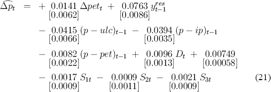
In (17), long-run homogeneity is imposed directly on the coefficients in the error correction term. This formulation emphasizes the effect on inflation of the disequilibrium in the long-run mark-up equation, i.e., (2). Alternatively, long-run unit homogeneity may be imposed by re-arrangement of the variables within the ECM in (17), obtaining (21).

For comparison with (17), White's (1980) heteroscedasticity-consistent standard errors appear in square brackets [·]; see also MacKinnon and White (1985). Three distinct feedback terms appear in (21): (p – ulc)_t–1, (p – ip)_t–1, and (p – pet)_t–1, each with its coefficient estimated unrestrictedly. These feedbacks are the negative logs of lagged real unit labour costs, real import prices, and real energy costs; cf. (4). These real prices are comparisons of nominal sectoral prices with the CPI, and so are also relative prices involving the price being explained by the equation. As such, these real prices focus attention on existing disequilibria of the domestic goods market relative to the domestic labour market, the foreign goods market, and the energy market. This interpretation is in the spirit of Juselius's (1992) model of Danish inflation and Metin's (1994) model of Turkish inflation, both of which examine the effects that numerous intra-and inter-sectoral disequilibria have on inflation. Franz and Gordon (1993) find strong error correction feedbacks for models of German and American producer price indices, as does Ericsson (1994) for the U.S. consumer price index although, in both these studies, the error correction appears to be simply real unit labour costs. Because (21) is isomorphic to (17), the remainder of this paper refers to (17) alone, except when the representation in (21) is required.

6.3 Statistical Properties of the Model

The statistical properties of the model can be assessed by what is not modelled, namely, the residuals. Residuals from full-sample and subsample estimates are both informative. Using a battery of residual diagnostic test statistics, this subsection shows that (17) appears well-specified, with empirically constant coefficients.

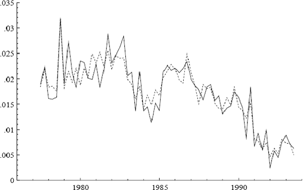
As noted in Section 5.2, the preferred equation performs well in terms of standard (full-sample) diagnostic tests. Empirically, the residuals are normally distributed, homoscedastic, and serially uncorrelated; and the null hypothesis of no omitted variables is easily accepted for a wide variety of variables. Figure 14 plots the actual and fitted values for Δp_t and shows how well (17) explains the data.

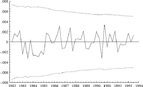
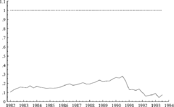
Estimation over subsamples by a recursive algorithm provides an incisive tool for investigating constancy; cf. Brown, Durbin and Evans (1975) and Dufour (1982). Graphs efficiently summarize the large volume of output. Figures 15 and 16 portray two related functions of the residuals from recursive estimation: the first summarizes the numerical constancy of (17) and the second its statistical constancy. Figure 15 records the one-step residuals and the corresponding calculated equation standard errors for (17), i.e., and in a common notation. The equation standard error varies little, declining slightly over time. Figure 16 plots the “break-point” Chow (1960) statistics for the sequence {1982(1)–1993(3), 1982(2)–1993(3), 1982(3)–1993(3), ..., 1993(2)–1993(3), 1993(3)}. None of these Chow statistics is significant at even their one-off 5% levels. That is, there is no break of the sample into estimation and forecast periods such that the corresponding Chow statistic for predictive failure is significant.

Recursive estimates of individual coefficients in (17) vary little, both numerically and statistically. The estimates' stability provides additional evidence that the right-hand side variables in (17) are weakly exogenous for the parameters in this equation, in which case single equation estimation is valid and without loss of information relative to the VAR. Appendix 2 considers these recursive estimates in detail.

The empirical stability of (17) suggests that the inflationary process in Australia has remained largely unchanged during the 1980s and 1990s, even while inflation itself has declined. This stability exists in spite of known changes to institutions and economic structure over the period. The explanation for the decline in inflation, therefore, lies in what happened to actual nominal wages and labour productivity, the exchange rate, prices for Australia's trading partners, tariffs, petrol prices, and the output gap.

6.4 Caveats

Some caveats apply to this analysis of inflation, although their empirical import may be minimal. First, the model makes no allowance for recent increases in indirect taxes. Because the parameter estimates in (17) are very stable over time, one would then expect these tax increases to affect the residual of (17). Yet, the residuals over 1992–1993 have been typical in magnitude. As a potential explanation, difficult trading conditions may have forced domestic producers and retailers to absorb some of the tax effects. Second, the mark-up on imports between the dock and the final point of sale may have fallen recently with increased market openness and competition, as discussed in Dwyer and Lam (1994) and Dwyer and Romalis (1995). While the model in (17) includes a measure of the tariff rate, it has no variables that would account for additional such changes in the mark-up. From the statistical properties of (17), the consequences to (17) of such changes appear small empirically.

Footnotes

For a permanent change in unit labour costs, import prices, or the output gap, the proportion of adjustment through to period n is (or zero for n = 0), where c₁ is the coefficient on the error correction term in (17). The cumulative adjustment for petrol prices is somewhat more complicated algebraically, but it is easily computed. For instance, for a 1% permanent increase in petrol prices, the contemporaneous effect on the CPI is 0.0141%, which is approximately 15% (= 0.0141/0.092) of the total long-run 0.092 percentage point effect on the CPI. [10]

The normalized distributional properties for ulc_t, ip_t, and are identical because each variable enters (17) at one and the same lag (the first). [11]