
RDP 2026-03: Shock-percentile Restrictions for SVARs 4. Estimating Noise in Beta SOFIA
June 2026
- Download the Paper 3,250KB
Our main goal is to understand how market characteristics and different benchmark construction techniques affect the amount of noise in Beta SOFIA. Noise in the repo market can be understood as transactions that do not reflect current market conditions. A recurrent example is when a repo transaction is part of a larger trade, where the individual transactions may not reflect the current market condition, but together they are meaningful. For example, a cross-currency swap trade that includes a repo trade in the home market, a swap into the foreign currency, a repo trade in the foreign market and a swap back into the home currency. Another example is netted packages, which include a repo transaction in one maturity and a reverse repo in another maturity, such that the participant is long in one maturity and short in another (Hempel et al 2023). In both cases, individual transactions may be treated as noise if considered separately.
To measure noise empirically, we decompose the observed Beta SOFIA rates into information and noise. We use a simple local-level state-space model where the observed benchmark is the sum of an efficient benchmark rate, mt, and a transitory pricing error, st.
Following Menkveld et al (2007), the efficient component is assumed to follow a random walk, implying that innovations to the efficient rate have a permanent effect on its level:
where mt–1 is the efficient rate on day t –1, and wt is information incorporated into the efficient rate on day t. The pricing error, st, is assumed to iid – independent and identically distributed – such that it only affects the current value of Beta SOFIA (and so is transitory by definition). The data-generating process for the observed benchmark rate, yt, is a sum of the efficient rate, mt, the pricing error, st, and control variables, xt, specifically the RBA's cash rate target:
State-space methods allow efficient decomposition of yt into information (wt) and noise (st) while controlling for the cash rate target. As is standard in many state-space applications, both st and wt are assumed to be normally distributed with mean zero and variances and respectively. The assumption of normality allows us to apply a standard Kalman filter to get maximum likelihood estimates of wt and st for each period.
As per Brugler et al (2025), we use the exact diffuse prior for the initial conditions and the L-BFGS algorithm to maximise the log-likelihood function and constrain all variance terms to be no smaller than 10–7. Each model is estimated twice, with maximum iterations of 1,000 and 10,000 respectively, to verify convergence and robustness of the results.
We use the model described in Equations (1) and (2) to extract the daily pricing error term, st, and take its absolute value as our definition of noise, such that noise increases on days with larger (absolute) values of st.
First, we estimate the model on Beta SOFIA calculated using ASX methodology and run time series regressions where the dependent variable is the noise term. The explanatory variables are repo market characteristics such as total volume, liquidity, market concentration, and amount of related-party transactions.
Next, we compare the transaction-level repo rates with the efficient level of Beta SOFIA, as determined by the model. This allows us to construct a transaction-level noise estimate, defined as the absolute difference between the repo rate on a transaction and the efficient rate.
Lastly, we use the underlying transaction data to construct hypothetical SOFIA benchmarks based on different computational rules and compare the aggregate (mean) noise in hypothetical SOFIAs with the published Beta SOFIA. This allows us to assess the benefits of different trimming techniques or criteria for the use of expert judgement.
On average, Beta SOFIA exhibits a daily noise level of 0.45 basis points, with substantial variation across time (standard deviation of 0.62 and a maximum of 9.67 – see row 1 of Table 1). The average transaction-level noise is 1.5 basis points with a standard deviation of 2.34 basis points. While most transactions exhibit small deviations, some extreme outliers persist, with a maximum deviation approaching 300 basis points (see row 1 of Table 2).
4.1 Aggregate determinants of benchmark noise
Our time series analysis allows us to estimate the conditional correlation between benchmark noise and market characteristics at the daily level. After estimating the absolute value of the noise term, st, from the state-space model, we regress it on daily market structure variables. Specifically, we estimate the following regression model:
where Noiset is the absolute value of noise on day t, RelPartyt is the number of related-party transactions on day t, and HHIt is a measure of market concentration, calculated using dollar volumes in the repo market. The vector Controlst includes some market characteristics: transaction volume (measured as log dollar volume of all daily transactions), and liquidity (measured by three variables: Amihud ratio – a measure of the price impact of trades; Hui-Huebel ratio – a measure of the resilience dimension of liquidity; and bid-ask spreads on 3-year government bonds). The error term ut captures any other factors that may influence noise but are not explicitly included in the model.
The regression results in Table 3 suggest that benchmark noise increases with:
- the number of related-party transactions, then is positive; and
- higher market concentration, that is, when trading activity is more concentrated and only a few counterparties are present in the market, then is positive.
| (1) | (2) | (3) | (4) | (5) | (6) | (7) | |
|---|---|---|---|---|---|---|---|
| No of related-party transactions | 0.005** (0.002) |
0.005** (0.002) |
0.004* (0.002) |
0.003 (0.003) |
0.005** (0.002) |
0.007** (0.003) |
|
| HHI | 6.26*** (1.50) |
6.23*** (1.48) |
6.24*** (1.48) |
5.87*** (1.55) |
6.24*** (1.49) |
7.53*** (1.58) |
|
| Bid-ask 3-year | 7.44 (6.82) |
||||||
| Hui-Huebel ratio | 2.82** (1.38) |
||||||
| Amihud ratio | 0.001 0.001 |
||||||
| Market volume | 0.097** (0.048) |
||||||
| Observations | 803 | 803 | 803 | 803 | 803 | 802 | 803 |
| R2 | 0.004 | 0.089 | 0.11 | 0.094 | 0.124 | 0.13 | 0.13 |
|
Notes: ***, ** and * denote statistical significance at the 1, 5 and 10 per cent levels, respectively. Newey-West standard errors with five lags are in parentheses. Sources: ASX; Authors' calculations; Bloomberg. |
|||||||
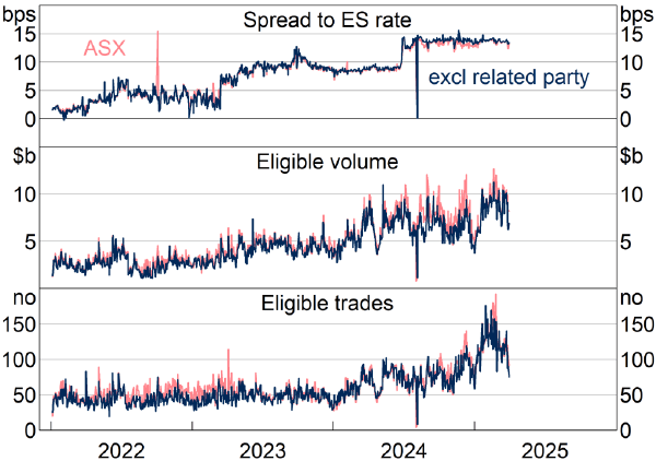
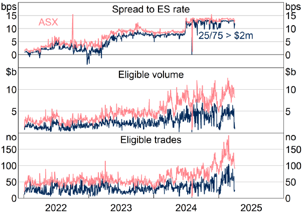
These findings suggest that related-party transactions and market concentration are detrimental to our measure of benchmark efficiency. To illustrate the effects of related-party transactions on Beta SOFIA, Figure 3 compares Beta SOFIA with a synthetic version constructed by excluding related-party transactions.
Note: ES rate is the remuneration rate on exchange settlement balances (which are internationally called reserves) banks receive on their excess reserves.
Sources: ASX; Authors' calculations.
4.2 Transaction-level determinants of benchmark noise
In addition to market-level analysis, we examine noise at the transaction level. This more granular approach allows for a richer econometric specification that can control for observed and unobserved characteristics (through fixed effects) of transactions or market-wide effects. We estimate the following regression model:
where Noisei,b,t is the absolute value of noise for the transaction between seller i buyer b on day t. RelPartyDummyi,b,t is the dummy variable taking the value of 1 if seller i and buyer b are related parties, MarketSharei,b,t is the share of dollar volume of this transaction relative to the total dollar volume on day t. Controlsi,b,t is a vector of control variables that includes transaction volume, buyer fixed effects, seller fixed effects, day fixed effects, and collateral-day fixed effects.
The collateral-day fixed effects allow us to compare noise in trades that are executed on the same day and with the same type of collateral. Although all Beta SOFIA-eligible transactions are backed by high-quality liquid assets (HQLA), there are some differences between Australian Government and state government debt securities which could lead to different pricing. For example, for international banks, Australian Government securities qualify as HQLA for liquidity regulation purposes, but state government securities do not. The heterogeneity in the quality of collateral may affect repo pricing and noise. Therefore, in regression specifications with collateral-day fixed effects, we compare noise in transactions within the same collateral class and macro-market conditions, thus reducing omitted variable bias in these regressions.
The results in Table 4 indicate that related-party transactions are associated with higher benchmark noise, consistent with time series analysis. The estimated coefficients for the related-party dummy are positive and significant across all model specifications. This points to the fact that related-party transactions are also detrimental to benchmark efficiency.
| (1) | (2) | (3) | (4) | (5) | (6) | |
|---|---|---|---|---|---|---|
| Related-party dummy | 1.14*** (0.13) |
0.12*** (0.0003) |
1.14*** (0.13) |
0.15*** (0.03) |
||
| Market share | 3.16*** (0.45) |
15.15*** (0.86) |
3.17*** (0.46) |
15.31*** (0.87) |
||
| Transaction volume | –0.03*** (0.004) |
0.07*** (0.006) |
–0.06*** (0.005) |
–0.05*** (0.007) |
–0.06*** (0.005) |
–0.05*** (0.008) |
| Buyer fixed effects | Y | N | Y | N | Y | N |
| Seller fixed effects | Y | N | Y | N | Y | N |
| Day fixed effects | Y | N | Y | N | Y | N |
| Collateral-day fixed effects | N | Y | N | Y | N | Y |
| Observations | 53,153 | 35,661 | 53,153 | 35,661 | 53,153 | 35,661 |
| Within R2 | 0.004 | 0.01 | 0.003 | 0.041 | 0.007 | 0.043 |
|
Notes: ***, ** and * denote statistical significance at the 1, 5 and 10 per cent levels, respectively. Standard errors are in parentheses and clustered on the collateral-day dimension. Sources: ASX; Authors' calculations. |
||||||
Higher market share, that is, concentration, is also associated with increased noise, which reinforces the idea that market dominance can lead to one or several large trades swaying the benchmark rate. In contrast, larger transaction volume is negatively associated with noise, suggesting that smaller trades contribute more to benchmark variability.
Overall, the panel data findings align with our time series results: benchmark noise is elevated in less competitive, more concentrated markets, and in the presence of related-party activity. These results are based on estimates from regressions that compare transactions within the same day (day fixed effects), controlling for different buyers and sellers and within the same day and the same collateral type (collateral-day fixed effects).
4.3 Benchmark design features and noise
We now explore whether alternative versions of Beta SOFIA could improve benchmark quality. While the 25th percentile trim has been retained, this reflects its distinct purpose of excluding transactions priced below prevailing cash funding rates due to collateral-driven demand, rather than addressing statistical noise. Our focus is therefore on addressing potential noise at the upper end of the rate distribution. Bottom-end trimming is widely adopted across major benchmarks such as SOFR, SONIA, CORRA and €STR, whereas practices around top-end trimming remain less standardised and continue to evolve. Therefore, we focus on different forms to account for noise on the top end of the distribution. To do this we construct several synthetic SOFIAs by (i) adjusting the trimming parameters and (ii) excluding small trades below the threshold of $2 million. Specifically, we test the following synthetic variations:
- 25/95th percentile trimmed mean
- 25/95th percentile trimming, excluding transactions below $2 million
- 25/75th percentile trimmed mean
- 25/75th percentile trimming, excluding transactions below $2 million
- 25th percentile trimming, excluding transactions with price above mean plus two standard deviations.
After computing each synthetic SOFIA, we estimate a modified version of the state-space model, which compares the synthetic rates' noise to that in actual Beta SOFIA (which employs a trimming approach that excludes the bottom 25 per cent of volume after sorting the rates from lowest to highest).[7] The state-space model assumes that both benchmarks follow a single efficient rate that itself follows a random walk as in Equation (1). Each observed Beta SOFIA variant is the sum of this efficient benchmark and a variant-specific noise term, , which are mean zero, iid normal with variance . The data-generating process for variant is:
where refers to different rates calculated using transaction data from date t. The model for Beta SOFIA and a variant rate can be jointly written in state-space form as:
where yt =(yt,1, yt,2)′, I2 is the 2×2 identity matrix, xt is the RBA cash rate target, is a vector of constants, one of which is normalised to zero, that capture persistent spreads between variants, is a 2×1 vector of pricing errors with distribution and H is a 2×2 diagonal matrix with and on the diagonal elements.[8] We can again employ standard state-space methods to estimate wt and for = 1,2 via maximum likelihood. Estimation details are as per Section 4.1. The variance of the pricing errors, and specifically, their relative magnitudes, are the key outputs of the model. We define the noise share of benchmark as:
A noise share of 50 per cent implies both benchmarks are equally noisy, while less than 50 per cent implies that that the benchmark has lower noise than the alternative.
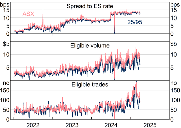
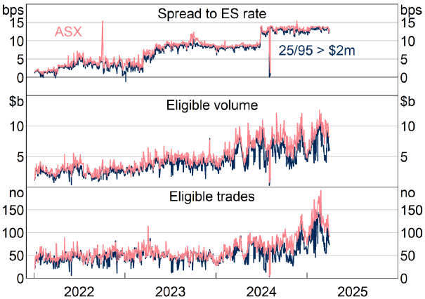
Table 5 reports the noise share associated with each trimming approach. We find that applying a 25/95th percentile trimmed mean results in a statistically significant reduction in benchmark noise, lowering the noise share from 0.58 in baseline Beta SOFIA to 0.42 in the synthetic version. This corresponds to a reduction of 16 percentage points and is significant at the 1 per cent level (Figure 4). Going a step further and taking small transactions out of the sample (> $2 million) does not result in further improvement (Table 5 and Figure 5). Thus, selecting transactions based on their transaction volume does not deliver a more efficient rate in the Beta SOFIA methodology.
| Beta SOFIA | Synthetic SOFIA | Difference | |
|---|---|---|---|
| 25/95th percentile | 0.58 | 0.42 | 0.16*** |
| 25/95th percentile, > $2million | 0.57 | 0.43 | 0.14*** |
| 25/75th percentile | 0.52 | 0.48 | 0.04 |
| 25/75th percentile, > $2million | 0.52 | 0.48 | 0.04 |
| 25th percentile/mean + 2 std dev | 0.75 | 0.25 | 0.50*** |
|
Notes: Difference tested with Wald test. ***, ** and * denote statistical significance at the 1, 5 and 10 per cent levels, respectively Sources: ASX; Authors' calculations. |
|||
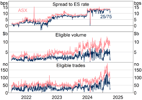
Narrower trimming (25/75) produces more modest noise reduction, with noise shares of 0.52 for baseline Beta SOFIA versus 0.48 for the variant, regardless of trade size threshold. However, the volume reduction is substantial (Figures 6 and 7). Narrower trimming, which reduces the upper bound from the 95th to the 75th percentile while retaining the bottom trim at the 25th percentile, also affects the level of the rate because the distribution is skewed. This raises the question of bias. While the bottom trim primarily removes transactions priced below prevailing cash funding rates due to collateral-driven demand, top-end adjustments aim to reduce noise without distorting the efficient rate. Our results indicate that narrower trims do not provide a less biased estimate of the efficient rate. These differences are not statistically significant.
Sources: ASX; Authors' calculations.
Sources: ASX; Authors' calculations.
Sources: ASX; Authors' calculations.
Sources: ASX; Authors' calculations.
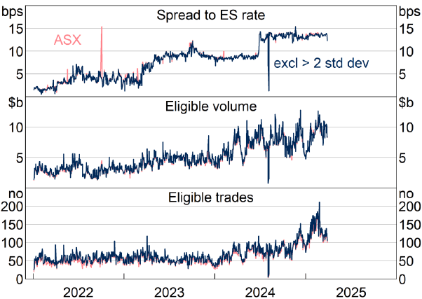
As an alternative to percentile trimming, we propose an extreme values trim that excludes all prices above the daily mean plus two standard deviations (Figure 8). This method excludes only 222 observations in total and because these tend to be extreme values the method performs better overall. It corresponds to a noise reduction of about 50 percentage points. Although this methodology performs better statistically it presents some challenges. Because the share of observations excluded in each day changes, this methodology might be perceived as less transparent. To the best of our knowledge, no reference rate trims extreme value observations based on standard deviations. Under the current ASX methodology, this form of trimming is not directly supported, as trimming is applied after sorting the data by price. Accordingly, for this study, the cut-off rate and standard deviation were calculated prior to trimming.
Sources: ASX; Authors' calculations.
Overall, the results suggest that Beta SOFIA can reduce its noise by trimming the top end of the distribution. A trade-off emerges in the implementation of such a trim. On one hand, a small trim at the top (such as the 95th percentile) is easily traceable and follows commonly used strategies. On the other hand, excluding only the observations that are above mean plus two standard deviations reduces noise by a greater amount without loss of too many observations. With these results the administrator can balance out which form a trim in the top end of the distribution can take.
4.4 Expert judgement thresholds
Our analysis in Sections 4.1 to 4.3 suggests that low-volume, low-transaction and high-concentration days tend to be associated with high levels of noise. Therefore, a natural next step is to assess whether there are (and if we can identify them) threshold values of volume, number of participants and number of transactions below which the Beta SOFIA noise spikes. These threshold values are particularly relevant for identifying low-liquidity environments in which the benchmark may require expert judgement.
In our observation window, the days with particularly low transaction volumes are NSW-only public holidays, that is, Labour Day and the Bank Holiday.[9] On these days, settlement occurs but transaction volume is very low because many banks are closed or operating with limited staff. According to communication with the ASX, the administrator will consider only transactions where the second leg of the trade takes place on the business day after the holiday going forward, that is, SOFIA will not be formed on these days. Nevertheless, these days present a useful experiment to understand how noise is related to liquidity and so we conduct our analysis without the ASX's proposed adjustments.
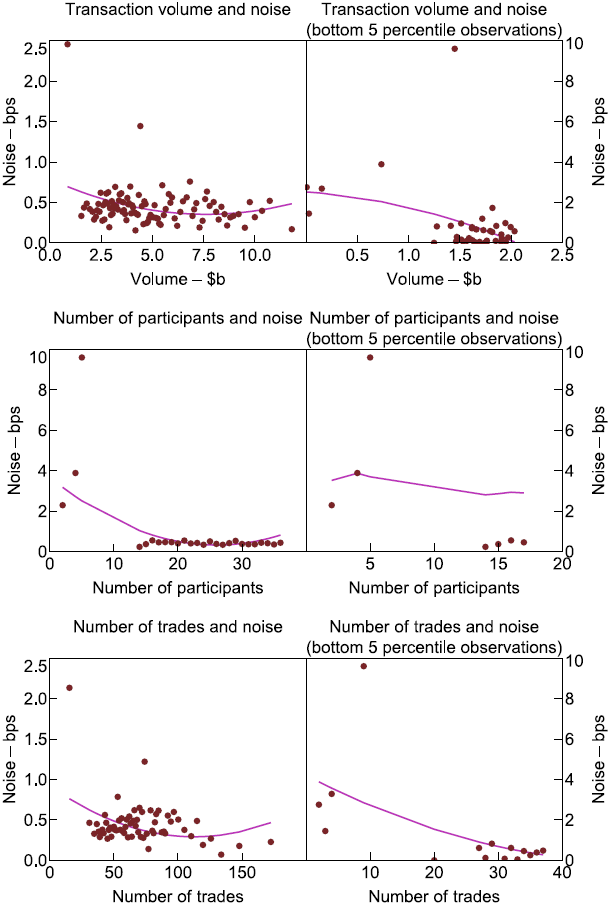
We examine the relationship between transaction volume and noise using binned scatter plots, where each point represents 1 percentile of noise on the y-axis and volume, number of participants or number of transactions on the x-axis (Figure 9). Binned scatter plots only show one observation per value on the x-axis. In this case, the dots shown are the average of different values on the y-axis. The left-hand panels present the full sample, while panels on the right hand zoom in on the bottom 5 percentile of the volume/number of participants/number of trades distribution. A sharp deterioration in benchmark quality is observed once transaction volumes fall below approximately $0.75 billion. Similarly, we observe a sharp increase in noise when the number of market participants is below 6 and when there are fewer than 12 transactions in the market. This nonlinear pattern suggests that noise becomes disproportionately elevated in less liquid market conditions, consistent with theoretical predictions that market depth and participant diversity enhance benchmark robustness.
Sources: ASX; Authors' calculations.
To validate this threshold empirically, estimate the following regression:
We define the dummies in the following ways:[10]
- Dummy 1: ≤ $0.1 billion and ≤ 3 trades (2 observations);
- Dummy 2: ≤ $0.5 billion and ≤ 10 trades (3 observations);
- Dummy 3: ≤ $1.2 billion and ≤ 15 trades (4 observations);
- Dummy 4: ≤ $1.5 billion and ≤ 20 trades (5 observations);
- Dummy 5: ≤ $1.5 billion and ≤ 30 trades (6 observations); and
- Dummy 6: ≤ $1.75 billion and ≤ 40 trades (12 observations).
Noiset is the absolute value of noise on day t, log(Volume)t is the natural logarithm of dollar volume of transactions on day t, and the dummy variables are defined at the thresholds of liquidity specified above.
The results in Table 6 suggest that noise is significantly higher on low-volume, low-transaction-number days compared to days with above $1.5 billion volume and 20 trades. The largest marginal increase in noise comes from the transactions in the bucket of $1.2 to $1.5 billion volume and below 20 trades.
As a robustness check we investigate if the spike in noise shown in Figure 9 is still present once we account for the administrator's new methodology, that is, removing NSW labour days and bank holidays. We find no such spike (see Figure A1). Thus, we conclude that at values higher than the threshold, calculated noise does not seem to spike.
| (1) | (2) | (3) | (4) | (5) | (6) | |
|---|---|---|---|---|---|---|
| log(Volume) | –0.162** (0.082) |
–0.124 (0.079) |
–0.069 (0.049) |
0.069 (0.087) |
0.027 (0.092) |
–0.067 (0.064) |
| Dummy 1 | 0.713 (0.561) |
|||||
| Dummy 2 | 1.235** (0.582) |
|||||
| Dummy 3 | 1.965*** (0.445) |
|||||
| Dummy 4 | 3.899*** (1.432) |
|||||
| Dummy 5 | 3.058** (1.526) |
|||||
| Dummy 6 | 1.320 (0.996) |
|||||
| F-statistic | 10.74 | 12.86 | 11.93 | 4.86 | 5.68 | 7.74 |
| Observations | 803 | 803 | 803 | 803 | 803 | 803 |
|
Notes: ***, ** and * denote statistical significance at the 1, 5 and 10 per cent levels, respectively. Standard deviations are in parentheses. Sources: ASX; Authors' calculations. |
||||||
Footnotes
We also tested no trim SOFIA and bottom 40th percentile trim. Both were less efficient than the 25th percentile trim. [7]
For example, if one variant excludes the top 5 per cent of transactions by repo rate, it will have a positive average spread on another variant that is computed otherwise identically. [8]
In Australia, public holidays on one state may not necessarily occur on the same date as in other states. [9]
In parentheses, we describe the number of observations each dummy variable has equal to one. [10]