Research Discussion Paper – RDP 2025-08 Ageing and Economic Growth in China
November 2025
1. Introduction
China's ageing population is often seen by commentators as one of the primary factors weighing on China's medium- to long-term economic growth prospects (e.g. Yiu et al 2023; Bicker 2024). The demographic challenge is also often cited as a reason for pessimism over long-term fundamental housing demand, and therefore as a factor expected to gradually reduce China's demand for materials used in construction, such as steel (Baird 2024). This paper seeks to test these assumptions by constructing quantitative estimates for how ageing affects economic growth in China, as well as the extent to which different sectors are expected to be affected by an increase in population ageing.
To do so, this paper applies the instrumental variable approach of Maestas, Mullen and Powell (2023) (hereafter ‘MMP’) to Chinese data in order to estimate the decadal effect of ageing on GDP per capita. A popular approach in the literature has previously been to estimate the effect of ageing on growth by estimating panel regressions of GDP per capita growth on the change in the old-age ratio in Chinese provincial data (Song and Gao 2022; Jiang and Zhao 2023; Yan, Li and Pan 2023; Yang, He and Chen 2023).[1] However, directly regressing growth on population ageing is potentially a problematic approach due to confounding variables such as internal migration, which is likely responsive to provincial growth, and life expectancy, which is likely to increase more rapidly in faster growing provinces.
To counter these kinds of unobserved variable bias in a study on US ageing and growth, MMP use the ‘predetermined component’ of population ageing in US states as an instrumental variable for ageing. This predetermined component is the growth in the old-age ratio that would be implied by the state's population structure in a prior period, aged forward to present. This paper applies the same instrumental variable approach to Chinese provincial-level data from national censuses between 1982 and 2020. Using this approach, I estimate the effect of ageing on nominal GDP per capita growth, as well as the effect of ageing on the contribution of services and construction to GDP.
Using this instrument, I find that population ageing has a negative and significant impact on nominal GDP per capita growth. Specifically, a 10 per cent increase in the proportion of the population aged over 60 (e.g. from 20 to 22 per cent of the population) leads to a 7.2 per cent decrease in nominal GDP per capita in the baseline specification. Applying this estimate to the national level requires some caution, as the provincial panel approach cannot account for common national policy changes in response to population ageing or general equilibrium effects of national ageing. But with these caveats in mind, the estimates in this paper imply that China's GDP per capita growth would have been more than a quarter higher in the 2010s, absent any increase in the old-age ratio.
These estimates suggest that the ageing population has already had a significant impact on economic growth in China and will continue to do so in the coming decades. However, the decline in growth in China since the 2000s has also been much larger than the contribution of ageing implied by these estimates. That is, demographic change is an important factor for China's growth prospects, but does not explain the majority of the slowing in China's growth rate.
1.1 Background and literature
China's old-age population is increasing relatively rapidly, with the proportion of the population aged over 60 expected to increase by more than a third over the 2020s. China's fertility rate has declined sharply since the mid-2010s, with the country experiencing a notable decline in fertility in recent years, including relative to other countries with ageing populations (Figure 1). The United Nations's (UN's) latest population projection scenarios now imply a significantly higher dependency ratio in the long-term, exacerbating the potential consequences of the demographic transition identified in prior literature (Cai and Lu 2013; Lim and Cowling 2016). The UN's 2022 baseline dependency ratio projection runs close to what was considered to be a low-fertility scenario in 2015 (Figure 2).
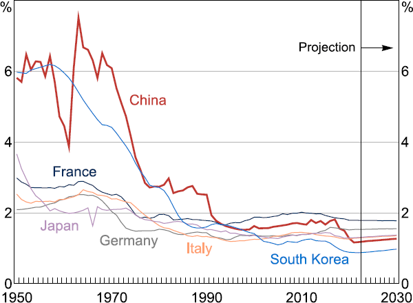
Source: UN World Population Prospects 2022.
Economic commentators generally believe ageing to have a negative effect on economic growth (IMF 2019; Cai 2021; Mason, Lee and Park 2022). An ageing population may be expected to put downward pressure on labour supply through a decreasing proportion (or even outright decline) of the working-age population, a decreasing support ratio (the ratio of workers to consumers), and decreasing labour productivity growth through factors such as decreasing investment (especially in infrastructure) due to reduced demand and potentially reduced political willingness. Population ageing may also lead to increased taxation being needed to finance old-age pensions and less flexible allocation of resources in the economy, such as through a less adaptable workforce to new technologies or to sectoral reallocation.
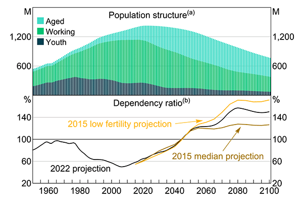
Notes:
(a) Youth is defined as 0–14 years, aged is defined as over 55 years for females and over 60 years for
males.
(b) Ratio of non-working-age to working-age population.
Sources: Author's calculations; Lim and Cowling (2016); UN World Population Prospects 2022.
However, theory does not guarantee a negative effect on growth per capita. The decrease in labour availability could also cause businesses to increase investment in technology, which could theoretically lead to a net increase in GDP per capita (Acemoglu and Restrepo 2017). That is, increased capital expenditure and labour productivity due to technological upgrading could outweigh the decline in the labour force and labour productivity resulting from the ageing population. For the most part though, the international empirical literature tends to find that the technology-upgrading effect is only a partial offset, and the overall effect of ageing on growth per capita is negative (Aksoy et al 2019; IMF 2019; Bodnár and Nerlich 2022; MMP).
As in the international literature, there are a mix of views in the Chinese academic literature, though most of the evidence finds a negative effect of ageing on China's economic growth (see Ni, Chen and Qiu (2014) for a literature review). Cai (2021) argues that demographic change may weigh on China's growth through: reducing demand for infrastructure and business investment; labour shortages and wage inflation, leading to the loss of traditional comparative advantage in labour-intensive exports; and declining consumption growth.
1.2 Approach
As discussed above, prior literature has attempted to address the question of how ageing affects per capita growth in China by estimating panel regressions of GDP per capita growth on the change in the old-age ratio in Chinese provincial data. This approach suffers from potential unobserved variable bias through factors that may relate to both ageing and growth, such as internal migration and life expectancy.
For example, suppose a negative trade shock hit a trade-exposed province, which caused a decline in economic growth due to reduced trade receipts. This shock may also induce younger workers to move to another province for work. This negative trade shock would therefore induce a correlation between economic growth and the proportion of the old-age population in the province, which could be mistaken for causation running from a change in the old-age population. Indeed, migration has historically been positively correlated with provincial GDP growth, indicating that migrants may choose their destinations in a way correlated with provincial growth (Figure 3). Another source of bias could be the fact that increased economic growth may itself increase life expectancy and therefore the old-age ratio, which would induce a spurious positive correlation between ageing and growth. Supporting this concern, life expectancy has been positively correlated with provincial economic growth over the past two decades (Figure 4).
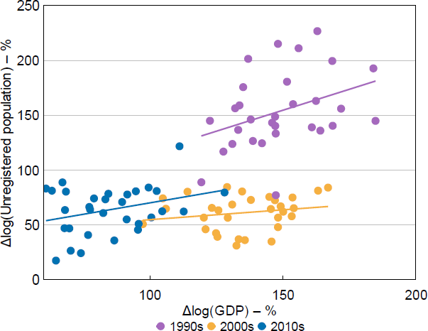
Note: Measures migration as the log difference in the ratio of the total usual population of the province to the population with household registrations in that province.
Sources: Author's calculations; CEIC Data; National Bureau of Statistics of China.
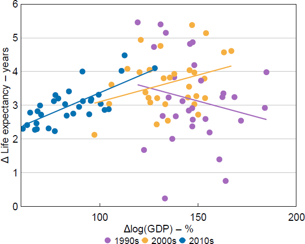
Sources: Author's calculations; CEIC Data; National Bureau of Statistics of China.
The approach in this paper applies the instrumental variable approach in MMP to Chinese data to counter these possible biases. The instrument in MMP is the predetermined component of ageing. Specifically, MMP use the US decadal censuses to estimate the effect of population ageing on growth over a 10-year period. For example, regressing states' GDP per capita growth on the change in the ratio of the population aged over 60 to the total population between 2000 and 2010, MMP would use as an instrument the change in the ratio of the population over 60 to the total population implied by a state's age distribution in 1990. MMP would age the 1990 distribution forward to 2000 and 2010 using the national-level survival rates. The idea behind this instrument is that this predetermined component of ageing should be correlated with realised ageing, but be sufficiently pre determined that it is uncorrelated with expectations of changing economic outcomes, or other shocks, in the decades ahead.
This paper is most closely related to Ye, Chen and Peng (2021), who also use the MMP instrumental variable approach for China, and find that a 10 per cent increase in the old-age ratio decreased real GDP per capita growth by 2 per cent over five years. This paper differs in that it uses a 10-year lag instrument (and 20- and 30-year lags for robustness) rather than only a 5-year lag in Ye et al (2021), and is therefore likely to be more robust to persistent shocks or endogenous expectations (see Section 2.3). It also uses 10-year rather than 5-year brackets of ageing and growth, comparable to MMP. Additionally, this paper has the benefit of the full decade of 2010–2020 census data rather than ending at 2015, as well as conducting additional sectoral exercises using the instrument in Section 4.[2]
2. Data, Methodology and Identification
2.1 Data
To apply this methodology for China, I collect province-level population counts by age from China's National Bureau of Statistics (NBS) census tabulations for the 1990, 2000, 2010 and 2020 censuses.[3] The 1982 census – the first of China's ‘reform and opening’ period – does not provide this tabulation publicly, so I estimate provincial population by age for 1982 using the IPUMS International 1 per cent sample of the microdata for the 1982 census (Ruggles et al 2024).[4] I collect NBS data on GDP per capita by province for 1990, 2000, 2010 and 2020 from the CEIC database.
I also collect the province-level proportion of employment by industry from the census for 1990, 2000 and 2010 for use as a time-varying control in the robustness checks described in Section 3.1.1. These employment figures are available from the 2000 and 2010 NBS tabulations, with a series of industry classifications that I summarise into four categories: agriculture, mining, manufacturing and other. As the 1990 Census industry-by-province employment is not available in the NBS tabulation, I use the IPUMS International 1 per cent microdata sample from the 1990 census to calculate the proportion of employment.
2.2 Methodology
As in MMP, I estimate the following regression of decadal log differences in GDP per capita on decadal log differences in the proportion of population aged over 60. In the regression, notation p indicates province, t is year, X is a set of time-varying control variables and is time fixed effects.[5] A is population aged over 60, and N is total population aged over 20.
I instrument the log differences in proportion of population over 60 with the predetermined component of ageing, using what MMP call a 20-year lag length – that is, I use the population structure at t −10, where t is the beginning year of the decade for which the effect on GDP growth is being estimated. The instrument is generated as:
where
and
Put plainly, for the 20-year lag instrument I calculate the predicted population over 60 at time t and t +10 by first multiplying the population in each province at time t −10 by the national level survival rate between t −10 to t and t +10, respectively, for the relevant age cohort. The national survival rates are calculated by taking the ratio of the total national age cohort at time t and t +10 compared to the size of the relevant age cohort at time t −10 (for example, the size of the 40–45 age cohort at time t on the size of the 30–35 cohort at time t −10 ). I then take the ratio of the predicted population aged over 60 at time t and t +10 and predicted total population aged over 20 for each province and period. The instrument is the log of the predicted population ratio over 60 at time t +10 subtracting the log of the predicted population ratio over 60 at time t.
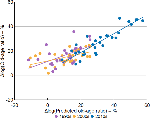
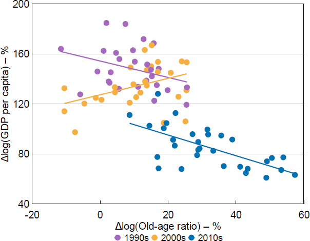
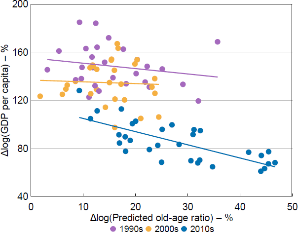
I illustrate the relationship between the instrument and actual ageing in Figure 5, between actual ageing and GDP per capita growth in Figure 6, and between the instrument and GDP per capita growth in Figure 7. Each dot represents a province, and the colour indicates the decade of the observation. Appendix A also includes map representations of the ageing data.
Sources: Author's calculations; CEIC Data; National Bureau of Statistics of China.
Sources: Author's calculations; CEIC Data; National Bureau of Statistics of China.
Sources: Author's calculations; CEIC Data; National Bureau of Statistics of China.
2.3 Identification
To meet the assumptions necessary for a valid instrumental variable, the instrument must be relevant, exogenous, and meet the exclusion assumption. The relevance assumption requires the instrument (predetermined component of the increase in population over 60) to be correlated with the key regressor (increase in population over 60). This would logically be true absent extreme levels of internal migration, and a weak instrument test rejects the hypothesis that the instrument is irrelevant.[6]
The exogeneity assumption requires that the instrument be uncorrelated with the error term . The exclusion restriction requires that the instrument does not affect economic growth except for through the instrumented variable: the actual change in the old-age ratio. The exogeneity and exclusion assumptions together require that a province's ‘past age structure affects future changes in economic outcomes only by affecting its subsequently realized age structure, and not through any other channel’ (MMP, p 313). For example, the predicted change in population should not be systematically correlated with exogenous shocks based on industry structure such as trade shocks. As another example, suppose slower growth in a region due to a negative demand shock induces higher mortality in the region, spuriously increasing the correlation between growth and the old-age ratio. Predicted ageing in the population should be uncorrelated with that negative demand shock.
A threat to the instrumental variable assumptions is if there is significant migration in a way that was systematically correlated with migrants' expectations for the province's economic growth between 10- and 20-years' time (not just the level of GDP per capita of the province at that time). While migrants undoubtedly make migration decisions on the basis of expectations for their labour market outcomes, which are in turn determined by the industry structure and growth prospects of the target province, until 2000 internal migrants in China overwhelmingly tended to be aged between 16 and 44 (NBS, UNFPA and UNICEF 2018), which is a somewhat less important cohort for identification in this model, as discussed below.
For the exogeneity assumption to hold, there also cannot be persistent shocks in the past that affect both predicted ageing (i.e. the population structure in the past) and growth in the future. While it is likely that factors such as natural resource allocation and the structural features of the Chinese political and economic system in the mid-20th century affect both population structures in the late 20th century and the level of development of a given province, it is less clear that these factors would affect the growth rate in a particular decade in the future. To illustrate the distinction, while GDP per capita in levels is highly correlated among provinces from decade to decade, the correlation between provincial GDP per capita growth in the 1990s and in the 2010s is actually slightly negative.[7] That is, even if households can, on average, predict provincial growth in the next decade, they may not necessarily correctly predict growth in the decade following that. To further account for potential identification issues, I explore the robustness of the estimates in Section 3 by stretching back the lag of the instrument to t – 20 and t −30. Increasing the time difference between the census used to generate the instrument and the observations in question should reduce the likelihood of expectations or persistent shocks playing a biasing role.
The MMP instrument is in spirit a Bartik, or ‘shift-share’ type instrument. The construction of these type of instruments can make interpretation of the identifying assumptions difficult. In this ‘shift-share’ instrument, the ‘share’ is the proportion of provincial population in each age cohort at t −10, and the ‘shift’ is the national-level cohort survival rates. To expound on where the identification originates in the MPP instrument, I follow Goldsmith-Pinkham, Sorkin and Swift (2020) in decomposing the Rotemberg weights of the equivalent GMM estimator with age cohort-by-province shares as instruments. These weights are interpretable as showing the components of the Bartik instrument to which the estimates are most sensitive to misspecification. That is, greater Rotemberg weights for an age cohort imply that the identification of the instrumental variables is more reliant on the variation in the proportion of population in that cohort between provinces.
The population cohort shares at t −10 which have the largest (absolute) Rotemberg weights are those cohorts which age into the over-50 category by time t, followed by the birth cohorts in the decade prior to t −10, which will age into the denominator of the old-age ratio (all people aged over 20) (Table 1). Put simply, the estimation approach can be thought of as mostly comparing the GDP per capita growth rates for t to t +10 between provinces with larger and smaller populations aged over 50 at t −10, as well as higher and lower birth rates between t −20 and t −10. The size of the population over 50 at t −10 would be determined by the province birth rate at time t −60 and earlier, and by migration decisions of people in that age cohort from anywhere between t −70 and t −10.
| Age cohort | Cohort share of population(a) | |
|---|---|---|
| 50+ | 0.375 | 0.187 |
| 0–9 | 0.296 | 0.145 |
| 40–49 | 0.176 | 0.135 |
| 10–39 | 0.154 | 0.524 |
|
Notes: Unlike in the canonical Bartik instrument where Rotemberg weights are usually positive, in this instrument some weights are negative by construction (increasing in size of cohorts which are only in the denominator of the old-age ratio subtracts from the ratio). I therefore present the weights as absolute weight on sum of absolute weights to give a clearer interpretation of cohort importance. (a) Average across provinces and years. |
||
3. Results
3.1 Main estimates
Estimating the regression using ordinary least squares (OLS) and without the instrument suggests that a 10 per cent increase in the proportion of the population aged over 60 is associated with a 2.7 per cent decrease in nominal GDP per capita and is not statistically significant (Table 2). Applying the instrument in the regression, the coefficient is increasingly negative and becomes highly statistically significant. With the instrument, I find that a 10 per cent increase in the proportion of the population aged over 60 leads to a 7.2 per cent decrease in nominal GDP per capita.[8] Following MMP, this functional form relies on per cent (rather than percentage point) changes in the old-age ratio, such that a 10 per cent increase in the old-age ratio here refers to, for example, an increase in the old-age ratio from 10 per cent to 11 per cent, or from 20 per cent to 22 per cent (I test a specification with percentage point changes below). As a point of reference, in the 2010s the old-age ratio increased around 3.6 per cent per year. Running the instrumental variable regression without the time-varying control for whether a province is coastal, the estimate is somewhat more negative, with a 10 per cent increase in the old-age ratio leading to around a 9 per cent decrease in GDP per capita.
| OLS | Instrumental variables | ||
|---|---|---|---|
| 20-year lag | 20-year lag | ||
| log(old-age ratio) | −0.270 (0.181) |
−0.716*** (0.210) |
−0.899*** (0.202) |
| Controls | |||
| Year | Y | Y | Y |
| Is Coastal | Y | Y | N |
| Is Coastal*Year | Y | Y | N |
| Observations: clusters | 84: 28 | 84: 28 | 84: 28 |
| Notes: ***, ** and * denote statistical significance at the 1, 5 and 10 per cent levels, respectively. Standard errors are in parentheses and clustered at a provincial level. | |||
Unlike in MMP, in which the OLS estimates are more negative than the instrumental variable estimates, the OLS estimates here appear to be biased towards zero. That is, there may be some unobserved variables inducing a spurious positive correlation between ageing and growth which is corrected by the instrument. For example, if economic growth substantially improves life expectancy, greater growth in a province leads to a greater proportion of the population living to an older age, increasing the old-age ratio. In comparison, MMP argue that the OLS is biased away from zero for the United States due to younger migrants choosing to migrate to higher growth states. Over the period of observation in this paper, China's life expectancy increased significantly faster than that of the United States in the MMP study. The bias induced by the positive correlation between life expectancy and growth may therefore have a larger effect in the Chinese data than in the US data. That is, it could be that the unobserved factors inducing a negative correlation for the United States are dominated by unobserved factors inducing a positive correlation in China.[9]
I also test four other specifications for robustness (Table 3). First, instead of controlling by geographic location, I follow MMP in controlling for initial industry employment shares by province, interacted with the time fixed effect. This allows for the possibility that provincial industry structure is systematically related to the prior population age structure and future GDP per capita growth. This is another way of getting at the possibility of persistent shocks affecting both industry structure and age structure, and therefore inducing a correlation between ageing and growth through the incidence of later industry-specific shocks. Second, instead of controlling by geographic location, I use province fixed effects, to account for the possibility of persistent fixed differences in trends between provinces. Third, I extend the instrument to be calculated at t −20 (i.e. a 30-year lag), which makes the possibility of the age structure at that time being systematically related to growth prospects in the decade under study more remote. Fourth, I extend the instrument to t −30 (a 38-year lag, given the 1982 Census timing), for the same reason. All four of these specifications return significant negative estimates for the effect of ageing on growth around the value of the main specification: ranging from a 5.7 per cent to an 8.7 per cent decrease in nominal GDP per capita in response to a 10 per cent increase in the proportion of the population aged over 60.
| 20-year lag | 20-year lag | 30-year lag | 40-year lag | ||
|---|---|---|---|---|---|
| log(old-age ratio) | −0.868*** (0.199) |
−0.569** (0.287) |
−0.615*** (0.182) |
−0.806*** (0.180) |
|
| Controls | |||||
| Year | Y | Y | Y | Y | |
| Industry | Y | N | N | N | |
| Industry*Year | Y | N | N | N | |
| Is Coastal | N | N | Y | Y | |
| Is Coastal*Year | N | N | Y | Y | |
| Province fixed effect | N | Y | N | N | |
| Observations: clusters | 84: 28 | 84: 28 | 58: 30 | 28: 28 | |
|
Notes: ***, ** and * denote statistical significance at the 1, 5 and 10 per cent levels, respectively. Standard errors are in parentheses and clustered at a provincial level. |
|||||
An additional consideration is whether the log difference on log difference functional form is the most appropriate. The implication of this functional form is that equal per cent changes in the old-age ratio have the same effect on economic growth, rather than equal percentage point changes. For example, by this assumption, a doubling in the old-age ratio from 5 to 10 per cent should have the same effect as a doubling from 10 to 20 per cent. Another way of estimating the equation would be as a log difference in GDP per capita on a difference in the old-age ratio. That is, estimating the effect of a percentage point change in the old-age ratio (e.g. an increase in the old-age ratio from 20 per cent of the population to 21 per cent of the population). Formally:
This specification yields qualitatively similar effects of ageing on growth. The effect of ageing on growth is negative and significant, and a 1 percentage point increase in the old-age ratio (which would be equivalent to a 10 per cent increase when the old-age ratio is 10 per cent of the total population, and a 5 per cent increase when the old-age ratio is 20 per cent) would decrease GDP per capita by 3.7 per cent (Table 4). However, this functional form would have slightly different implications for how China's national-level ageing will affect its economy in the coming years.
| 20-year lag | |
|---|---|
| log(old-age ratio) | −3.710*** (0.985) |
| Controls | |
| Year | Y |
| Is Coastal | Y |
| Is Coastal*Year | Y |
| Observations: clusters | 84: 28 |
|
Notes: ***, ** and * denote statistical significance at the 1, 5 and 10 per cent levels, respectively. Standard errors are in parentheses and clustered at a provincial level. |
|
3.2 Applying the estimates nationally
To understand what these estimates imply about China's macroeconomic trends and growth outlook, I next apply the estimates to national level data. This exercise requires caveats. As MMP point out, estimates derived from variation amongst sub-national units cannot account for the effects of national level policies, such as a nationwide increase in the retirement age, or an increase in pension payments. It also cannot account for general equilibrium effects of population ageing. For example, an increase in the older population beyond current levels could put increasing strain on the fiscal sustainability of old age pensions, which could cause a decrease in government spending elsewhere, thereby reducing economic growth through other channels. Ageing would likely also affect the balance of savings and investment, which would have implications for the neutral rate of interest and the exchange rate. The bias on these estimates when applied nationally could be upwards or downwards, as it depends on the nature of the policies and general equilibrium effects at play.
For this exercise, I take the estimate of the effect of ageing on growth as a 7.2 per cent decrease in nominal GDP per capita for a 10 per cent increase in proportion of population aged over 60 and apply it to the UN's national-level projections of the old-age ratio (Figure 8). From 1981 to 1990, when the old-age ratio declined by around 3 per cent, demographic change added around 2.3 percentage points to nominal GDP per capita growth compared to the counterfactual of no change. In contrast, between 2011 and 2020, population ageing detracted around 28 percentage points from nominal GDP per capita growth relative to the counterfactual of no growth in the old-age ratio, as a result of the old-age ratio increasing 39 per cent.
For comparison, China's nominal GDP per capita in practice grew by 98 per cent over that period. That is, the estimates imply that nominal GDP per capita growth would have been more than a quarter higher in the absence of any increase in the old-age ratio over 2011 to 2020. Or put differently, the estimates imply GDP per capita in 2020 to be around 12 per cent smaller than if the old-age ratio had not changed over the 2010s. Between 2021 and 2030, ageing would be expected to detract another 28 percentage points from nominal GDP per capita growth relative to the counterfactual of no increase in the old-age ratio.
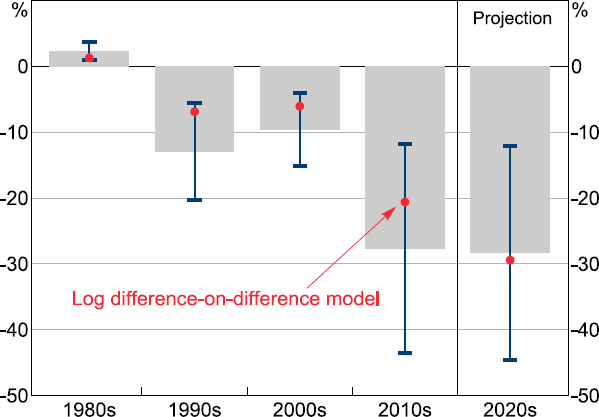
Notes: Effect of change in the old-age ratio on GDP per capita growth relative to a counterfactual of no change in the old-age ratio. Whiskers indicate 95 per cent confidence intervals.
Sources: Author's calculations; UN World Population Prospects 2022.
The implied reduction in GDP per capita growth in the 2010s is somewhat comparable to the reduction of potential output in OECD economies after the global financial crisis (Ball 2014).[10] The scale of the effect is testament to the importance of demographic structure for medium- to long-run economic growth. Another relevant illustration is the sizeable contribution to growth of the ‘demographic dividend’ that an expanding working-age population had for several east Asian economies in the 1970s (Mason et al 2022). However, it is also worth noting that China's nominal GDP per capita grew 253 per cent over the 2000s, meaning the overall decline in GDP per capita growth between the 2000s and 2010s was more than five times the amount of the decline that could be explained by the effect of ageing.
The 95 per cent confidence interval around this estimate suggests that the reduction of growth over the 2020s could be between 12 and 45 percentage points. An alternative approach would be to use the log-differences on differences functional form, discussed above. Over both the 2010s and the 2020s the old-age ratio is projected to increase by around a third. But in percentage point terms, the increase over the 2020s would be larger, implying that the effect of ageing on growth – shown as dots in Figure 8 – will increase from around 21 per cent in the 2010s to 29 per cent in the 2020s, rather than being about the same. Both estimates imply that ageing will have a large effect on growth in the 2020s relative to a counterfactual of no increase in the old-age ratio.
3.3 Implications
While these projections suggest a challenging demographic outlook for the economy, demographics are not necessarily destiny. Lim and Cowling (2016) point out that the economic effects of an increase in the dependency ratio driven by population ageing could be offset by policies that: increase the fertility rate, increase the retirement age, improve total factor productivity (TFP), increase the urbanisation rate, or increase the participation rate.
One approach to offsetting the demographic decline would be to directly attempt to reverse, or slow the decline through pro-natalist policies. Authorities have introduced policies designed to increase the birth rate such as by lifting the limit on the number of children a family can have, introducing financial and administrative incentives to have children in certain regions and seeking to address factors which increase the cost of child rearing (Department of Education, Skills and Employment 2022; Ji 2023). These approaches have failed to lift fertility so far, and the UN Population Division continues to project that fertility will not return to the levels of the early 2010s (Cai 2021; United Nations Population Division 2024). However, media have recently reported the possibility of wider-ranging support in the future directly from the central government to families with more than one child (Reuters 2024), and authorities have also introduced a nationwide childcare subsidy (Xinhua 2025). A step-up in support from the central government could impact fertility decisions more than incentives previously administered at the local government level.
Another approach to slowing the decline in the working-age population is to increase the retirement age. After rumours that such a policy was under consideration for some years, China adopted new legislation in September 2024 to gradually increase the statutory retirement age over the course of 15 years starting from 2025 (Zhao 2021; Reuters 2023; Xinhua 2024). The change entails an increase in the statutory retirement age from 60 to 63 for men, 55 to 58 for white-collar women, and 50 to 55 for blue-collar women. This policy, although gradual, could imply that the effect of ageing on growth in the future may be slightly smaller than estimated in this paper as the retirement age increases.
Rather than directly offsetting the decline in growth through demographic policies, another approach would be to attempt to keep growth stable by pursuing policies that would increase growth, all else equal. In particular, TFP improvements could play this role, with researchers identifying increasing human capital and continued urbanisation as a potential boon for China's productivity (Cai and Lu 2013; Marois, Gietel-Basten and Lutz 2021). The average years of schooling received by China's working-age population is expected to increase significantly over coming decades, as the cohorts newly entering the workforce are much higher educated than the cohorts leaving the workforce. Additionally, the rapid mechanisation of China's industrial production, and increasing focus on high-tech industries which are less labour intensive, are a salient source of growth in the capital stock, and potentially TFP growth. Indeed, China's top authorities have signalled that this approach, along with expanding services segments that serve the elderly population – the ‘silver economy’ – will be important aspects of the policy response to the ageing population (Xi 2024).
The risk of this kind of structural change is that it could increase the wage gap between more- and less-educated workers (especially between rural and urban labour; see, for example, Rozelle and Boswell (2021)). That is, although the average education will increase, the returns from this increase in human capital may disproportionately go to the highest educated, leaving behind less-educated cohorts, especially rural residents. Indeed, this kind of inequality could further inhibit consumption growth in China, in line with literature that argues that increased income inequality can be growth-inhibiting (Cingano 2014). Authorities could mitigate these concerns by improving the social safety net, thereby unleashing high household savings (Cai 2021).
Urbanisation is another continuing positive trend for China's productivity and growth. The productivity of China's urban labour force is substantially higher than for the rural population (reflecting factors such as industrial structure, health and educational attainment), and the process of urbanisation brings with it increased consumption and investment (IMF 2019). China's urbanisation rate of around 66 per cent is still well below that of developed countries, which tend to have urbanisation rates around 80 per cent or above.
However, despite the tailwinds of education, urbanisation and the increasing technological complexity of manufacturing, improving productivity growth in China remains a challenge. Similar to global trends, productivity growth in China has been in secular decline. In the Chinese context, researchers and international organisations variously attribute the slowing to declining business dynamism, resources misallocation between state-owned and private firms, a reduction in the exit of inefficient state-owned firms, and reduced efficiency of capital usage (particularly in infrastructure) (Brandt et al 2022; Cerdeiro and Ruane 2022; IMF 2023). That is, further structural reforms are needed to ensure expanding TFP growth and capital accumulation if authorities seek to exert upward pressure on China's growth rate at a time when demographics are pushing down potential growth.
4. Sectoral Divergence
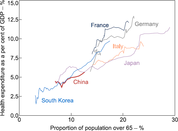
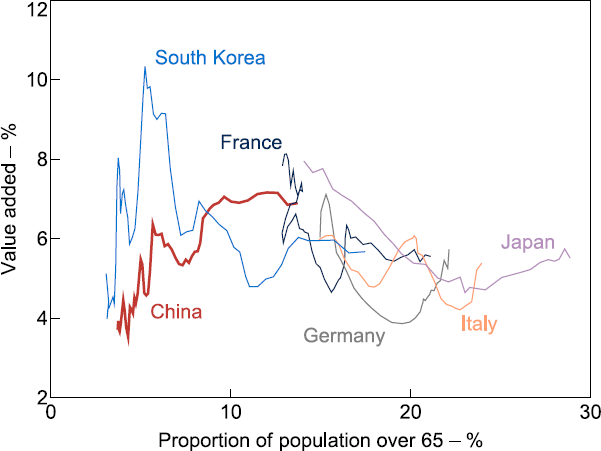
Looking beyond the aggregate economic effect of the ageing population, demographic trends are likely to have divergent effects on different sectors of the economy. Sectors for which an ageing population would increase demand, such as health care, are generally expected to be beneficiaries, whereas sectors that have previously benefited from a fast-growing population, like real estate, are expected to suffer. This is borne out in the experience of countries further along in their ageing process such as France, Germany, Italy, Japan and South Korea. As these countries have aged, health expenditure as a proportion of GDP has generally risen, while value added by the construction sector as a proportion of total value added has mostly declined (Figures 9 and 10).
Sources: Author's calculations; OECD.
Note: Includes both residential and non-residential construction.
Sources: Author's calculations; OECD.
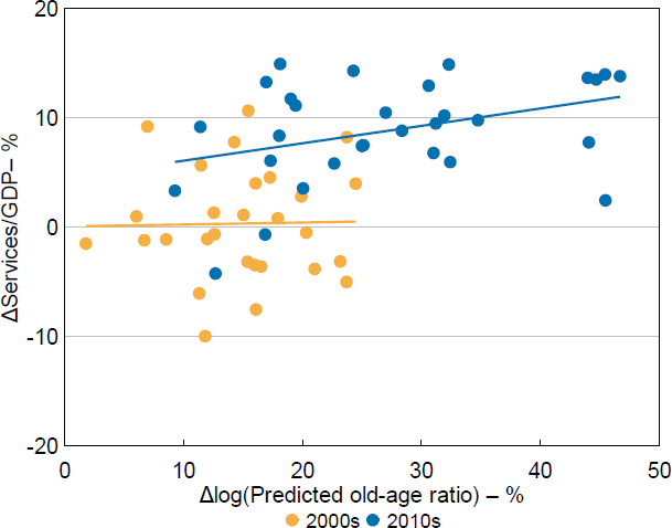
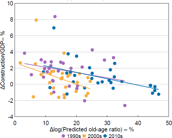
To test whether this is also the case for China, I take the panel approach described above, and replace GDP per capita as the dependent variable with sectoral contributions to GDP. In particular, I examine the effect of ageing on the proportion of provincial GDP that is contributed by the services sector (excluding real estate services), and the proportion contributed by construction. Formally, I estimate:
where Sector is services (excluding real estate) or construction. I again estimate this equation using decadal data to align with the census years, and construct the 20-year lag instrument in the same way described in Section 2.2. While I am able to estimate this equation for the construction sector contribution for each of the decades between 1990 and 2020, China's provinces only began reporting real estate services (which is needed to construct services excluding real estate) in their GDP data in 1992. I therefore estimate the model for the effect on services excluding real estate from 2000 onwards. I illustrate the relationship between the ageing instrument and each of these measures in Figures 11 and 12.
Note: Line of best fit shown for each decade.
Sources: Author's calculations; CEIC Data; National Bureau of Statistics of China.
Note: Line of best fit shown for each decade.
Sources: Author's calculations; CEIC Data; National Bureau of Statistics of China.
As might be expected, these regressions suggest that an increase in the proportion of population aged over 60 results in an increase in the contribution of services to provincial GDP, with a 10 per cent increase in the proportion of the population over 60 leading to around a 1 percentage point increase in the sector's contribution to GDP (Table 5). On the other hand, an increase in the proportion of population aged over 60 leads to a 1 percentage point decrease in the contribution of construction to GDP. This aligns with the intuition that as the population ages, the structure of consumption shifts more towards services (such as health and aged care), while there is less need for new residential and infrastructure construction, as the formation of new households slows and the need for newly built infrastructure declines.
Applying these point estimates to China's national projected ageing trajectory would imply that the contribution of the services sector (excluding real estate) to national GDP could increase from its 2023 level of 48.7 per cent to 51.7 per cent by 2030. The construction sector's contribution would fall further from its 2023 level of 6.8 per cent to 3.6 per cent by 2030, using these estimates. In short, although China's demographic outlook poses a long-term headwind for the construction sector, it creates new opportunities to supply goods and services demanded by the ageing population.
| Services (excluding real estate) | Construction | |
|---|---|---|
| log(old-age ratio) | 0.099* (0.053) |
−0.104*** (0.031) |
| Controls | ||
| Year | Y | Y |
| Is Coastal | Y | Y |
| Is Coastal*Year | Y | Y |
| Observations: clusters | 58: 30 | 85: 30 |
|
Notes: ***, ** and * denote statistical significance at the 1, 5 and 10 per cent levels, respectively. Standard errors are in parentheses and clustered at a provincial level. |
||
5. Conclusion and Implications for Australia
The estimates in this paper suggest that among China's provinces an increase in the old-age ratio leads to lower nominal GDP per capita growth compared to if there had been no such increase. Applying these estimates nationally suggests that the projected increase in China's old-age population over the coming decade will act as a headwind to growth. However, there are policy options available for authorities to somewhat cushion this impact on the economy. Authorities have so far responded with policies which may help slow the decline in the working-age population, such as increasing the retirement age and introducing policies aimed at increasing the birthrate. Authorities have also signalled possible productivity-enhancing reforms which could put upward pressure on economic growth to counteract the negative impact of ageing on growth. Additionally, not all sectors stand to lose from the demographic transformation. These estimates suggest that while ageing poses a headwind to the construction sector, this trend may lead to an increase in the contribution of the services sector to the economy.
The Australian economy has previously been a significant beneficiary of Chinese commodity demand, especially for use in the construction sector. The estimates in this paper suggest that shifting demographics are likely to reduce demand for these kind of exports to China from Australia in the coming decades. However, there remain opportunities for countries such as Australia to benefit from a growing share of services consumption in China, including through business opportunities in market segments that serve the elderly population in China, such as health and aged care.
Appendix A: China Data and Regressions
A.1 Geographic variation
The following maps illustrate the log differences in old-age ratio by province. Figure A1 shows the data for the 1990s, Figure A2 for the 2000s and Figure A3 for the 2010s.
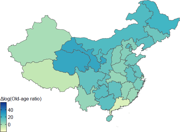
Sources: Author's calculations; CEIC Data; National Bureau of Statistics of China.
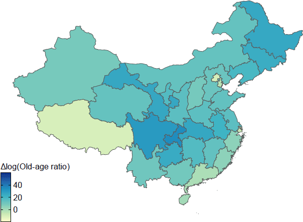
Sources: Author's calculations; CEIC Data; National Bureau of Statistics of China.
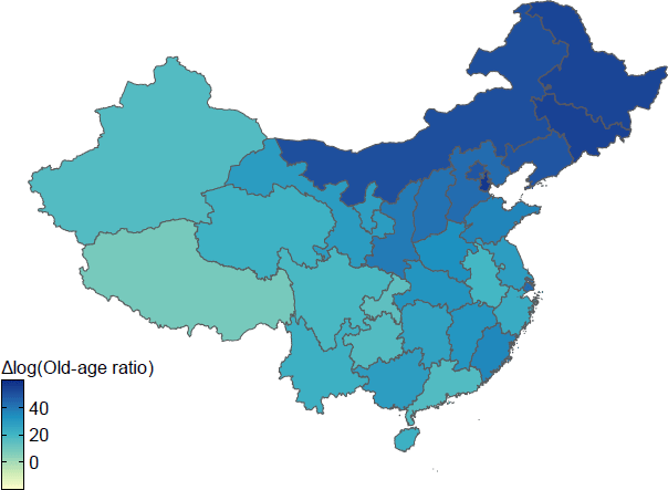
Sources: Author's calculations; CEIC Data; National Bureau of Statistics of China.
A.2 Intertemporal growth correlations
As discussed in Section 2, the correlation between provincial growth over the 1990s and over the 2000s is negative. However, for the 2000s and 2010s, this correlation is positive.
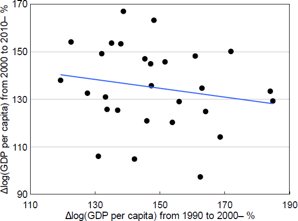
Note: Line of best fit shown.
Sources: Author's calculations; CEIC Data; National Bureau of Statistics of China.
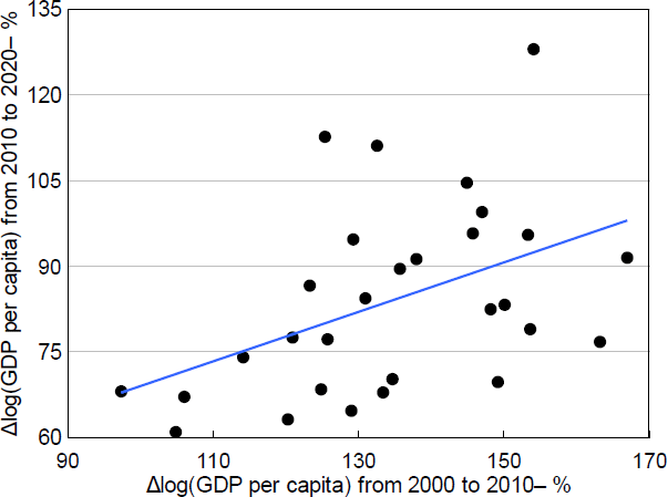
Note: Line of best fit shown.
Sources: Author's calculations; CEIC Data; National Bureau of Statistics of China.
A.3 Full regression results
The first-stage regression summary statistics for the main specification are shown in Table A1.
| R-squared | Adjusted R-squared | Robust F (1,27) | Prob > F | |
|---|---|---|---|---|
| log(old-age ratio) | 0.7675 | 0.7493 | 70.6168 | 0.0000 |
|
Note: F-statistic adjusted for 28 clusters of provinces. |
||||
The full table for the regressions described in Tables 2 and 3 is shown in Table A2.
| OLS | Instrumental variables | ||||||
|---|---|---|---|---|---|---|---|
| 20-year lag | 20-year lag | 20-year lag | 20-year lag | 30-year lag | 40-year lag | ||
| log(old-age ratio) | −0.270 (0.181) |
−0.716*** (0.210) |
−0.899*** (0.202) |
−0.569** (0.287) |
−0.868*** (0.199) |
−0.615*** (0.182) |
−0.806*** (0.180) |
| Controls | |||||||
| Year | |||||||
| 2000 | 0.017 (0.059) |
0.651 (0.074) |
−0.114** (0.057) |
−0.120** (0.056) |
−0.101 (0.240) |
||
| 2010 | −0.427*** (0.073) |
−0.337*** (0.074) |
−0.427*** (0.068) |
−0.506*** (0.092) |
−0.889*** (0.177) |
−0.382*** (0.053) |
|
| Industry | |||||||
| Agriculture | 0.159 (0.121) |
||||||
| Mining | −0.027 (0.021) |
||||||
| Manufacturing | 0.198*** (0.065) |
||||||
| Industry#Year | |||||||
| Agriculture#2000 | 0.206* (0.111) |
||||||
| Agriculture#2010 | −0.167 (0.122) |
||||||
| Mining#2000 | 0.043 (0.043) |
||||||
| Mining#2010 | 0.044 (0.033) |
||||||
| Manufacturing#2000 | −0.143* (0.075) |
||||||
| Manufacturing#2010 | −0.254*** (0.070) |
||||||
| Coastal | |||||||
| Coastal | 0.229*** (0.049) |
0.207*** (0.047) |
−0.158** (0.074) |
−0.130*** (0.041) |
|||
| Coastal#2000 | −0.363*** (0.079) |
−0.372*** (0.084) |
|||||
| Coastal#2010 | −0.382*** (0.068) |
−0.340*** (0.063) |
0.022 (0.075) |
||||
| Province fixed effects | N | N | N | Y | N | N | N |
| Constant | 1.416*** (0.027) |
1.468*** (0.032) |
1.567*** (0.036) |
1.634*** (0.034) |
1.969*** (0.144) |
1.482*** (0.058) |
1.160*** (0.077) |
| Observations: clusters | 84: 28 | 84: 28 | 84: 28 | 84: 28 | 84: 28 | 58: 30 | 28: 28 |
| Notes: ***, ** and * denote statistical significance at the 1, 5 and 10 per cent levels, respectively. Standard errors are in parentheses and clustered at a provincial level. | |||||||
Running the main specification of the instrumental variable regression individually for each decade shows that the coefficient on ageing is large and negative for the 2000s and 2010s, and smaller for the 1990s (Table A3). The sample size when running the regression using individual decades is relatively small.
| Decade | Effect of GDP per capita growth |
|---|---|
| 1990s | −0.053 (0.785) |
| 2000s | −0.768 (0.693) |
| 2010s | −0.895*** (0.171) |
|
Notes: ***, ** and * denote statistical significance at the 1, 5 and 10 per cent levels, respectively. Standard errors are in parentheses and clustered at a provincial level. |
|
The full table for the regression described in Table 4 is shown in Table A4.
| 20-year lag | |
|---|---|
| log(old-age ratio) | −3.710*** (0.985) |
| Controls | |
| Year | |
| 2000 | 0.036 (0.062) |
| 2010 | −0.306*** (0.079) |
| Coastal | |
| Coastal | 0.226*** (0.046) |
| Coastal#2000 | −0.376*** (0.083) |
| Coastal#2010 | −0.336*** (0.067) |
| Constant | 1.439*** (0.029) |
| Observations: clusters | 84: 28 |
|
Notes: ***, ** and * denote statistical significance at the 1, 5 and 10 per cent levels, respectively. Standard errors are in parentheses and clustered at a provincial level. |
|
Appendix B: Sectoral Regressions
The full table for the regressions described in Table 5 is shown in Table B1.
| Services (excluding real estate) | Construction | |
|---|---|---|
| log(old-age ratio) | 0.099* (0.054) |
−0.104*** (0.031) |
| Controls | ||
| Year | ||
| 2000 | −0.013** (0.006) |
|
| 2010 | −0.058** (0.025) |
0.007 (0.009) |
| Coastal | ||
| Coastal | 0.030** (0.014) |
−0.019** (0.008) |
| Coastal#2000 | −0.019 (0.030) |
0.011 (0.008) |
| Coastal#2010 | 0.018** (0.008) |
|
| Constant | 0.045** (0.019) |
0.035*** (0.007) |
| Observations: clusters | 58: 30 | 85: 30 |
|
Notes: ***, ** and * denote statistical significance at the 1, 5 and 10 per cent levels, respectively. Standard errors are in parentheses and clustered at a provincial level. |
||
References
Acemoglu D and P Restrepo (2017), ‘Secular Stagnation? The Effect of Aging on Economic Growth in the Age of Automation’, The American Economic Review, 107(5), pp 174–179.
Aksoy Y, HS Basso, RP Smith and T Grasl (2019), ‘Demographic Structure and Macroeconomic Trends’, American Economic Journal: Macroeconomics, 11(1), pp 193–222.
Baird A (2024), ‘Urban Residential Construction and Steel Demand in China’, RBA Bulletin, April.
Ball L (2014), ‘Long-term Damage from the Great Recession in OECD Countries’, European Journal of Economics and Economic Policies, 11(2), pp 149–160.
Bicker L (2024), ‘China's Ageing Population: A Demographic Crisis Is Unfolding for Xi’, BBC.com, 2 April, accessed 27 June 2024. Available at <https://www.bbc.com/news/world-asia-china-68595450>.
Bodnár K and C Nerlich (2022), ‘The Macroeconomic and Fiscal Impact of Population Ageing’, ECB Occasional Paper No 296.
Brandt L, J Litwack, E Mileva, L Wang, Y Zhang and L Zhao (2022), ‘Recent Productivity Trends in China: Evidence from Macro- and Firm-level Data’, China: An International Journal, 20(1), pp 93–113.
Cai F (2021), ‘A Tale of Two Sides: How Population Ageing Hinders Economic Growth in China’, China: An International Journal, 19(3), pp 79–90.
Cai F and Y Lu (2013), ‘Population Change and Resulting Slowdown in Potential GDP Growth in China’, China & World Economy, 21(2), pp 1–14.
Cerdeiro DA and C Ruane (2022), ‘China's Declining Business Dynamism’, IMF Working Paper No WP/22/32.
Cingano F (2014), ‘Trends in Income Inequality and its Impact on Economic Growth’, OECD Social, Employment and Migration Working Papers No 163.
Department of Education, Skills and Employment (2022), ‘“Double Reduction Plan” Reduces Homework and Off-campus Tutoring for Chinese School Students’, International Education Engagement Resource, 20 January.
Goldsmith-Pinkham P, I Sorkin and H Swift (2020), ‘Bartik Instruments: What, When, Why, and How’, The American Economic Review, 110(8), pp 2586–2624.
IMF (International Monetary Fund) (2019), ‘Macroeconomics of Aging and Policy Implications’, G-20 Background Note, 5 June.
IMF (2023), ‘People's Republic of China: 2022 Article IV Consultation—Press Release; Staff Report; and Statement by the Executive Director for the People's Republic of China’, IMF Country Report No 23/67.
Ji S (2023), ‘China Population: Cities Unveil New Childbirth Incentives as First Decline in More than 6 Decades Looms’, South China Morning Post online, 12 January, accessed 27 June 2024. Available at <https://www.scmp.com/economy/china-economy/article/3206420/china-unveils-new-childbirth-incentives-population-growth-set-turn-negative>.
Jiang D and Zhao W (2023), ‘The Impact of Aging Speed on China's Economic Growth-An Analysis from the Perspective of Economic Inputs’, 2023(08), pp 63-80.
Lim J and A Cowling (2016), ‘China's Demographic Outlook’, RBA Bulletin, June, pp 35-42.
Maestas N, KJ Mullen and D Powell (2023), ‘The Effect of Population Aging on Economic Growth, the Labor Force, and Productivity’, American Economic Journal: Macroeconomics, 15(2), pp 306-332.
Marois G, S Gietel-Basten and W Lutz (2021), ‘China's Low Fertility May Not Hinder Future Prosperity’, Proceedings of the National Academy of Sciences of the United States of America (PNAS), 118(40), e2108900118.
Mason A, S-H Lee and D Park (2022), ‘Demographic Change, Economic Growth, and Old-age Economic Security: Asia and the World’, Asian Development Review, 39(01), pp 131-167.
National Bureau of Statistics of China, United Nations Population Fund and United Nations Children's Fund (NBS, UNFPA and UNICEF) (2018), ‘Domestic Migrants in China (2018): Trends, Challenges and Recommendations’, Joint data project. Available at <https://china.unfpa.org/en/report/20190816>.
Ni C, Chen Y and Qiu X (2014), ‘A Review of Research on the Impact of Aging on Economic Growth in China’, 2014(09), pp 87-93.
Reuters (2023), ‘China to Raise Retirement Age to Deal with Aging Population – Media’, Reuters online, 14 March, accessed 27 June 2024. Available at <https://www.reuters.com/world/china/china-raise-retirement-age-deal-with-aging-population-media-2023-03-14/>.
Reuters (2024), ‘Exclusive: China to Issue $284 billion of Sovereign Debt This Year to Help Revive Economy’, Reuters online, 26 September, accessed 10 October 2024. Available at <https://www.reuters.com/markets/asia/china-issue-284-bln-sovereign-debt-this-year-help-revive-economy-sources-say-2024-09-26/>.
Rozelle S and M Boswell (2021), ‘Complicating China's Rise: Rural Underemployment’, The Washington Quarterly, 44(2), pp 61-74.
Ruggles S, L Cleveland, R Lovaton, S Sarkar, M Sobek, D Burk, D Ehrlich, Q Heimann and J Lee (2024), ‘IPUMS International: D020.V7.5’, Integrated Public Use Microdata Series, accessed 27 June 2024. Available at <https://www.ipums.org/about/citation>.
Song J and Gao C (2022), ‘The Impact of Aging on Economic Growth and its Mechanisms—From the Perspective of Labor Supply and Social Security Expenditure’, 2022(11), pp 1-18.
Staiger D and JH Stock (1997), ‘Instrumental Variables Regression with Weak Instruments’, Econometrica, 65(3), pp 556-586.
United Nations Population Division (2024), ‘World Population Prospects’, accessed 27 June 2024. Available at <https://population.un.org/wpp/>.
Xi J (2024), ‘Supporting Chinese-style Modernization with High-quality Population Development’, Qiushi, online, 2022(22). Available at <https://www.qstheory.cn/dukan/qs/2024-11/15/c_1130219268.htm>.
Xinhua (2024), ‘(China Economic Roundtable) China Focus: Raising Retirement Age a Proactive Response to Population Aging’, Xinhua, 14 September, accessed 10 October 2024. Available at <https://english.news.cn/20240914/65d3d69c9e6a4cf89dbee6a063db65f5/c.html>.
Xinhua (2025), ‘China's Nationwide Childcare Subsidy Program Opens for Applications’, Xinhua, 8 September, accessed 3 November 2025. Available at <https://english.news.cn/20250908/017d557a9dbd4dc385c24539bb4d530d/c.html>.
Yan F, Q Li and N Pan (2023), ‘Regional Differences and Spatial Effects of the Aging Impact on Economic Growth’, 2023(12), pp 103-112.
Yang J, F He and T Chen (2023), ‘Empirical Evidence on the Impact of Population Aging on Growth’, 2023(02), pp 125-129.
Ye J, Z Chen and B Peng (2021), ‘Is the Demographic Dividend Diminishing in China? Evidence from Population Aging and Economic Growth during 1990-2015’, Review of Development Economics, 25(4), pp 2255-2274.
Yiu P, G Li, CK Tan and M Obe (2023), ‘China's Aging Population Threatens a Japan-style Lost Decade’, Nikkei Asia online, 22 March, accessed 27 June 2024. Available at <https://asia.nikkei.com/spotlight/the-big-story/china-s-aging-population-threatens-a-japan-style-lost-decade>.
Zhao Y (2021), ‘China Rolls Out Detailed Plan to Raise Retirement Age, Deal with Aging Society’, Global Times online, 14 March, accessed June 2024. Available at <https://www.globaltimes.cn/page/202103/1218323.shtml>.
Acknowledgements
Thank you to Samual Nightingale, John Boulter and Michelle Wright for their comments on preliminary versions of this work. I am grateful to Lauren Johnston and Jonathon Hambur for their feedback on the paper. Thank you also to Sarah Hunter, Anthony Brassil, RBA Seminar and ER Coffee participants for their helpful feedback and suggestions. These are the views of the author and should not be attributed to the Reserve Bank of Australia. Any errors are the sole responsibility of the author.
Footnotes
In this paper, the old-age ratio refers to the population aged over 60 as a proportion of the total population. [1]
This paper also uses nominal GDP per capita rather than real GDP per capita as in Ye et al (2021). These estimates therefore also include the relative regional effects of population ageing on prices. [2]
The main regressions include all provincial-level administrative units except for Chongqing and Sichuan (since the two were split in 1997) and Hainan (which was split from Guangdong, a considerably more populous province, in 1988). [3]
Specifically, I calculate the proportion of the population by age in each province from the 1 per cent sample of the microdata and then multiply by the provincial aggregate population counts reported in the NBS census tabulation to construct aggregate provincial population by age. This induces a slight (but likely random) error in the age-by-province population counts for 1982. The 1 per cent sample includes around 11 million people. [4]
The time-varying controls in the baseline results are whether or not the province is coastal, and the coastal variable with a time interaction. I include these geographic controls to account for the possibility that the significant increase in trade after China's accession to the World Trade Organization (WTO) in the 2000s, which would accrue mainly to the coastal provinces, could affect the results. [5]
An F-test returns an F-statistic of 71 for the instrument, well above the rule of thumb that the F-statistic should be above 10 to avoid a weak instrument (Staiger and Stock 1997). See Appendix A. [6]
See Appendix A. This pattern would be expected if less-developed provinces are expected to catch up to the GDP levels of more-developed provinces over time. Between the 2000s and 2010s on the other hand, this correlation is positive. [7]
By comparison, MMP estimate that a 10 per cent increase in the old-age ratio decreases real GDP per capita by 5.5 per cent for the United States. [8]
Or more pessimistically, it could be that the instrument is better at purging unobserved variable bias that induces a positive correlation than that which induces a negative correlation. [9]
Ball (2014) estimates an 8.4 per cent loss of potential output for a weighted average of OECD economies after the global financial crisis. These estimates are not directly comparable to those in this paper: the Ball estimates are real aggregate growth rates over around eight years, whereas this paper examines nominal per capita rates over ten years. However, the comparison does illustrate the importance of long-run structural features of the economy, even compared to major macroeconomic demand shocks. [10]