RDP 2025-03: Fast Posterior Sampling in Tightly Identified SVARs Using ‘Soft’ Sign Restrictions 4. Numerical Illustration and Monte Carlo Experiments

This section illustrates how our method works and explores its efficiency relative to accept-reject sampling using a simple bivariate model as an example. This allows us to easily and transparently control the size of the identified set as well as visualise the performance of the algorithm. We first consider a case where the identified set is connected before illustrating the ability of our approach to navigate the more challenging circumstance where the identified set consists of disconnected parameter regions. We consider higher-dimensional models in the empirical applications (Section 5).

4.1 Connected identified set

Let y_t = (p_t, q_t)′ contain log price and quantity, and consider imposing the following pattern of sign restrictions on the impulse responses:^[13]

The restrictions imply that the first equation of the model can be interpreted as a supply curve and the second as a demand curve. The price elasticity of supply is $\omega \left(\varphi ,Q\right)\equiv -{e^{\prime }}_{1,2}{A}_0{e}_{1,2}/{e^{\prime }}_{1,2}{A}_0{e}_{2,2}=-{\left({\Sigma }_{tr}^{-1}{e}_{1,2}\right)}^{\prime }{q}_1/{\left({\Sigma }_{tr}^{-1}{e}_{2,2}\right)}^{\prime }q1$.^[14] Consider augmenting the sign restrictions with the elasticity restriction $\omega \left(\varphi ,Q\right)\le \overline{\omega }$ with $\overline{\omega }\ge 0$.

Let vech$\left({\Sigma }_{tr}\right)={\left({\sigma }_{11},{\sigma }_{21},{\sigma }_{22}\right)}^{\prime }$ and note that $𝒪$(2) can be represented as

where we leave it implicit that $\theta \in \left[-\pi ,\pi \right]$ (e.g. Baumeister and Hamilton 2015).

It can be shown that the sign restrictions generate the following identified set for $\theta$:

The upper bound of the identified set converges to zero as $\overline{\omega }\to \infty$ and to $\arctan \left({\sigma }_{22}/{\sigma }_{21}\right)$ (i.e. the lower bound) as $\overline{\omega }\to 0$. The elasticity restriction therefore provides a convenient way to explore the efficiency of our algorithm relative to accept-reject sampling as the size of the identified set changes.

To illustrate the sampling approach in this setting, we fix $\varphi$ and assume the goal is to draw from the uniform distribution over $𝒬\left(\varphi |S\right)$, which is equivalent to drawing $\theta$ from a uniform distribution over $I{S}_{\theta }\left(\varphi |S\right)$ (Baumeister and Hamilton 2015). The accept-reject algorithm can be interpreted as drawing $\theta$ from a uniform distribution over the identified set given the sign normalisations only, and rejecting draws of $\theta$ that violate the sign restrictions.^[15] In contrast, the slice sampler generates a Markov chain whose invariant distribution is the distribution over $\theta$ induced by $f_{\text{Δ}}\left(Z\right)$. For $\text{Δ}>0$, this distribution assigns positive density outside $I{S}_{\theta }\left(\varphi |S\right)$, so the slice sampler will return draws of $\theta$ outside of $I{S}_{\theta }\left(\varphi |S\right)$ with positive probability, though draws of $\theta$ within $I{S}_{\theta }\left(\varphi |S\right)$ will be sampled with higher probability. The resampling step then discards draws outside of $I{S}_{\theta }\left(\varphi |S\right)$ and reweights the remaining draws so that the resulting distribution is (approximately) uniform.

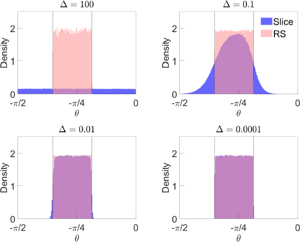
Figure 3 illustrates the sampler under different values of $\text{Δ}$.^[16] When $\text{Δ}$ = 100 (top left panel), which we take to approximate the behaviour of the algorithm as $\text{Δ}\to \infty$, values of $\theta$ that violate the sign restrictions are essentially not penalised. The slice sampler therefore generates draws of Q from a uniform distribution over $𝒪$(2), which corresponds to $\theta$ being uniformly distributed over the interval $\left[-\pi ,\pi \right]$. When $\text{Δ}=0.1$ (top right panel), values of $\theta$ that violate the sign restrictions have their density penalised, but a substantial proportion of draws obtained via slice sampling violate the sign restrictions. Values of $\theta$ that satisfy the sign restrictions but are close to the bounds of the identified set also have their density penalised, so the distribution of draws satisfying the sign restrictions is not uniform. Decreasing $\text{Δ}$ (bottom two panels) more strongly penalises values of $\theta$ that violate the sign restrictions, so a far smaller proportion of draws violate the restrictions, and the effective sample size following importance sampling is much larger. Following importance sampling, the draws are approximately uniformly distributed over $I{S}_{\theta }\left(\varphi \right)$.

To examine the computational efficiency of the sampling algorithms in this setting, we obtain 10,000 draws from $𝒬\left(\varphi |S\right)$ in each of 100 replications where the slice sampler is initialised at a different randomly generated value. We compute the average time taken to obtain the draws and the average effective sample size. If w_k is the importance weight attached to the kth draw, the effective sample size (expressed as a percentage of the original number of draws) is $ESS=\left(100/K\right)\times {\left({\Sigma }_{k=1}^K{w}_k\right)}^2/{\Sigma }_{k=1}^K{w}_k^2.$ To illustrate the trade-off between speed and effective sample size, we consider values of $\text{Δ}\in$ {0.1,0.01,0.001,0.0001} and $\overline{\omega }\in$ {1,0.1,0.01} (Table 1).^[17]

When $\overline{\omega }$ is relatively large, so that the identified set is ‘wide’, accept-reject sampling is more efficient than our approach, generating more effective draws in less time. As $\overline{\omega }$ decreases and the size of the identified set shrinks, the computational efficiency of our approach increases relative to accept-reject. For example, when $\overline{\omega }$ = 0.01, on average it takes 12.2 seconds to generate 10,000 draws using accept-reject, whereas the slice sampler with $\text{Δ}$ = 0.0001 generates around 9,700 effective draws in 1.3 seconds. For a given value of $\overline{\omega }$, increasing $\text{Δ}$ tends to increase computing time but also the effective sample size, since fewer candidate draws violate the sign restrictions.

4.2 Disconnected identified set

In general, $𝒬\left(\varphi |S\right)$ may be made up of disconnected regions. Sampling from a distribution that is supported on disconnected parameter regions can pose challenges for MCMC algorithms, because the Markov chain may become ‘stuck’ in one region and not adequately traverse the target distribution. In contrast, by virtue of its independent proposal density, the accept-reject algorithm does not suffer from this problem. In this exercise, we illustrate our sampling approach in a setting where the identified set is disconnected.

Consider imposing the restriction that the impulse response of the first variable to the second shock is weakly greater than some positive scalar: ${e^{\prime }}_{1,2}{A}_0^{-1}{e}_{2,2}={e^{\prime }}_{1,2}{\Sigma }_{tr}{q}_2\ge \lambda$ for $0\le \lambda \le {\sigma }_{11}$ (when $\lambda >{\sigma }_{11},I{S}_{\theta }\left(\varphi |S\right)=\left\{\text{∅}\right\}$ at any value of $\varphi$). All other impulse responses are unrestricted and we continue to impose the sign normalisation $\text{diag}\left(A_0\right)\ge 0_{2\times 1}$. This example nests Example B.5 in Giacomini and Kitagawa (2021b) when $\lambda =0$. When ${\sigma }_{21}<0$, the restrictions generate the following identified set for $\theta$:

which is the union of two disconnected intervals.^[18] For a given value of $\varphi$, the total length of the identified set shrinks with increasing $\lambda$. This example therefore provides a simple setting to illustrate our sampler when the identified set is disconnected.

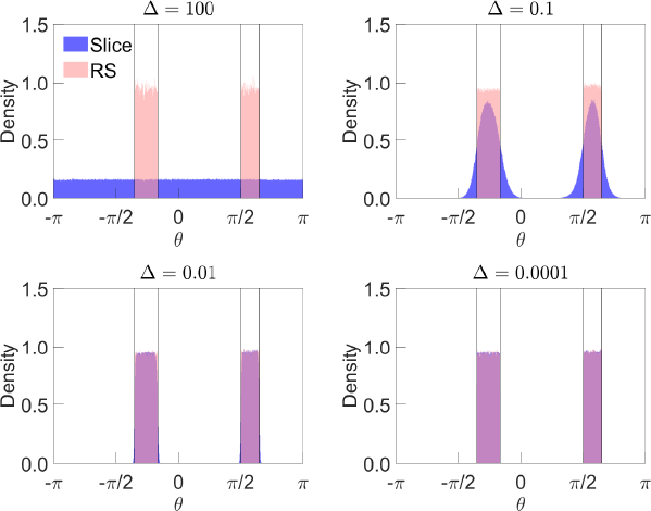
Figure 4 illustrates the sampler under different values of $\text{Δ}$. Even at small values of $\text{Δ}$, the sampler continues to cover the identified set – and thus generate draws from the target distribution – despite the identified set being disconnected. In the case where $\text{Δ}$ = 0.0001, 55.4 per cent of draws lie within the first interval, which is close to the theoretical probability under the uniform distriution (55.7 per cent). Our sampler therefore appears to adequately mix across the two regions.

These results point to the potential for our approach to improve the computational efficiency of posterior sampling under sign restrictions when the restrictions substantially truncate the identified set, even in cases where the identified set is disconnected. To assess whether the approach can deliver on this promise, in the next section we turn to a realistic empirical application.

Footnotes

These restrictions require ${e^{\prime }}_{1,2}{A}_0^{-1}{e}_{1,2}={e^{\prime }}_{1,2}{\Sigma }_{tr}{q}_1\ge 0$, ${e^{\prime }}_{2,2}{A}_0^{-1}{e}_{1,2}={e^{\prime }}_{2,2}{\Sigma }_{tr}{q}_1\le 0$ , ${e^{\prime }}_{1,2}{A}_0^{-1}{e}_{2,2}={e^{\prime }}_{1,2}{\Sigma }_{tr}{q}_2\ge 0$ and ${e^{\prime }}_{2,2}{A}_0^{-1}{e}_{2,2}={e^{\prime }}_{2,2}{\Sigma }_{tr}{q}_2\ge 0$. [13]

The price elasticity of supply is equivalently given by the impulse response of q_t to a demand shock that raises p_t by one unit (i.e. ${e^{\prime }}_{2,2}{A}_0^{-1}{e}_{2,2}/e_{1,2}{A}_0^{-1}{e}_{2,2}={e^{\prime }}_{2,2}{\Sigma }_{tr}{q}_2/{e^{\prime }}_{1,2}{\Sigma }_{tr}{q}_2$). [14]

In this example, the sign normalisations on the diagonal elements of A₀ are redundant given the sign restrictions. [15]

In this exercise, the slice sampler is initialised at a random draw of Z from a matrix standard normal distribution. [16]

The results are obtained using Matlab R2023a on a desktop computer running Microsoft Windows 10 Enterprise with an Intel Core i7-9700 CPU @ 3.00GHz, 8 cores and 128 GB RAM. [17]

This expression implicitly assumes $\lambda \le {\sigma }_{11}{\sigma }_{22}/\sqrt{{\sigma }_{22}^2+{\sigma }_{21}^2}$ otherwise the first interval is empty. [18]