RDP 2025-03: Fast Posterior Sampling in Tightly Identified SVARs Using ‘Soft’ Sign Restrictions 3. Algorithms

This section describes algorithms that can be used to obtain draws of Q from the uniform distribution over $𝒬\left(\varphi |S\right)$. We focus on sampling from this component of the posterior (or prior) distribution rather than the joint distribution of $\theta$, since the problem of sampling the reduced-form parameters is well understood (e.g. Del Negro and Schorfheide 2011). As a benchmark, we first describe an accept-reject algorithm. We then introduce our general approach to sampling based on ‘soft’ sign restrictions, before describing a specific MCMC sampler – the slice sampler – that can be used to implement our general approach.

3.1 Accept-reject sampling

The following algorithm describes an accept-reject sampler for drawing from the conditionally uniform distribution over $𝒬\left(\varphi |S\right)$.

Algorithm 1 (Accept-reject sampling). For a given value of $\varphi$:

Step 1. Draw an n×n matrix Z of independent standard normal random variables and let Z = $\tilde{Q}R$ be the QR decomposition of Z, where $\tilde{Q}$ is orthonormal and R is upper-triangular with non-negative diagonal elements.

Step 2. Normalise the signs of the columns of $\tilde{Q}$ such that $\text{diag}\left(A_0\right)\ge 0_{n\times 1}$ and let Q be the normalised matrix. If $\tilde{Q}=\left({\tilde{q}}_1,\mathrm{...},{\tilde{q}}_n\right)$, then

Step 3. Keep the draw if it satisfies $S\left(\varphi ,Q\right)\ge 0_{s\times 1}$ and terminate the algorithm. Otherwise, return to Step 1.

Step 1 draws $\tilde{Q}$ from a uniform distribution over $𝒪\left(n\right)$ using an algorithm proposed in Stewart (1980) (see also the descriptions in Rubio-Ramírez et al (2010) and Arias et al (2018)). Step 2 normalises the draw so that the sign normalisation diag$\left(A_0\right)\ge 0_{n\times 1}$ is satisfied, which increases the efficiency of the sampler relative to a sampler that omits this step and uses the subsequent accept-reject step to impose the sign normalisation.^[10] Step 3 is the accept-reject step, which simply involves checking whether the sign restrictions are satisfied. The algorithm is repeated to obtain the desired number of draws.

Let Q(Z) be a function that returns Q in the QR decomposition of Z (so Z = QR). Algorithm 1 can be interpreted as drawing Z from the truncated normal distribution with density

where f_Z(Z) is the density of the standard matrix normal distribution. The interpretation of Algorithm 1 as drawing from this density will be useful in introducing our sampler.

The challenge with using accept-reject sampling in this setting is that it may take a large number of candidate draws (and thus computational time) to obtain a sufficiently large number of draws satisfying the identifying restrictions. This will occur when $𝒬\left(\varphi |S\right)$ is assigned small measure under the uniform distribution over $𝒪\left(n\right)$ – that is, when identification is tight.

3.2 Soft sign restrictions

The indicator function $𝟙\left(Q\left(Z\right)\in 𝒬\left(\varphi |S\right)\right)$ appearing in Equation (7) can be decomposed into a product of indicator functions corresponding to individual sign restrictions:

where $𝒬\left(\varphi |S^{\left(l\right)}\right)=\left\{Q\in 𝒪\left(n\right):S^{\left(l\right)}\left(\varphi ,Q\right)\ge 0\right\}$ and $S^{\left(l\right)}\left(\varphi ,Q\right)\ge 0$ represents the lth sign restriction with l = 1,...,s. The key feature underlying our approach is that we replace the indicator function with a smooth regularisation (or penalty) function $\Lambda \left(f,\text{Δ}\right):ℝ\times {ℝ}_{+}\to \left(0,1\right)$, which satisfies the following assumption.

Assumption 1. The regularisation function $\Lambda \left(f,\text{Δ}\right)$ is such that

In addition, for some finite K > 0, it satisfies

for all $\text{Δ}\in {ℝ}_{+}$ and $f\in ℝ$.

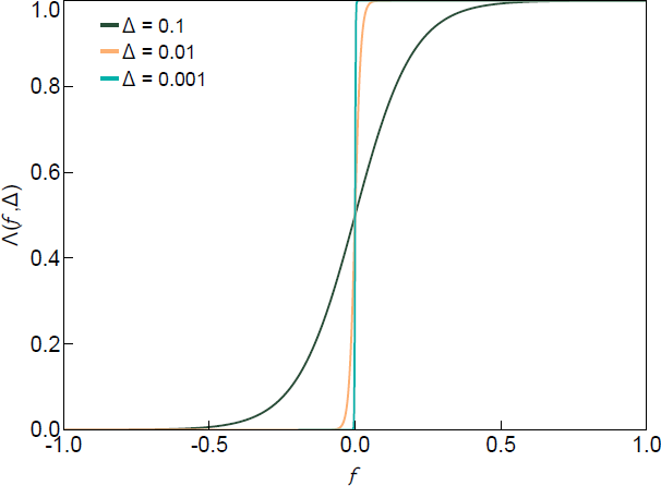
$\text{Λ}\left(f,\text{Δ}\right)$ can be interpreted as a function that penalises draws of Q (equivalently, Z) that violate (or are close to violating) the sign restrictions by down-weighting their density. In the limit as $\text{Δ}\to \text{0}$, the regularisation function converges to the indicator function. One choice for $\text{Λ}\left(f,\text{Δ}\right)$ that satisfies Assumption 1 (and that we will make use of below) is the logistic function:

This function is illustrated in Figure 1 for different values of $\text{Δ}$.

We propose sampling from a smooth density that replaces the indicator function with the regularisation function:

The advantage of working with this smooth density is that alternative sampling algorithms, such as MCMC methods, can be directly applied, which obviates the need for accept-reject sampling. In the limit as $\text{Δ}\to 0$, the probability of obtaining a draw violating the restrictions approaches zero and the draws of Q are approximately uniformly distributed over $𝒬\left(\varphi |S\right)$. This claim is formalised in the following proposition.

Proposition 1. Assume the conditions in Assumption 1 hold and let T : ${ℝ}^d\to ℝ$ be such that ${\displaystyle \int {}_{R^d}\left|T\left(Z\right)\right|f_{\text{Z}}\left(Z\right)dZ}<\infty$. Then,

where ${𝔼}_f(.)$ and ${𝔼}_{\text{Δ}}(.)$ are expectations taken under f and $f_{\text{Δ}}$, respectively.

For $\text{Δ}>0$, the obtained draws of Z will not necessarily satisfy the sign restrictions and – conditional on satisfying the sign restrictions – will not follow the desired truncated normal distribution; equivalently, the draws of Q will not be uniformly distributed over $𝒬\left(\varphi |S\right)$. However, an importance-sampling step can be applied to obtain draws from an approximation of the desired distribution. The importance weights are given by

We can compute these importance weights up to a normalising constant simply by evaluating the regularisation function and checking whether the sign restrictions are satisfied. The normalising constant is the ratio of the probability measures assigned to the identified set under the two probability distributions, and is computationally costly to obtain. An implication of ignoring this normalising constant is that the importance sampler draws from a distribution that is not exactly equal to $f\left(Z|Q\left(Z\right)\in 𝒬\left(\varphi |S\right)\right)$. However, a corollary of Proposition 1 is that the normalising constant converges to one as $\text{Δ}\to \text{0}$ (almost surely under the reduced-form prior). This implies that any bias present in the importance sampler should be small for small enough choices of $\text{Δ}$.

Theoretically, a smaller $\text{Δ}$ reduces the bias when approximating the posterior distribution of the structural parameters. However, a smaller $\text{Δ}$ also introduces sampling inefficiencies as the distribution becomes steeper (i.e. as the gradient of the log density function becomes larger). In the context of a random walk Metropolis algorithm, this steepness implies the need for a relatively smaller tuning parameter (i.e. the scale of the proposal distribution) to achieve a reasonable acceptance rate, as larger steps are more likely to be rejected in regions with high gradient changes. In the next section, we discuss an alternative method – slice sampling – that is more robust in such situations, offering improved efficiency in navigating steep target distributions.

Finally, if the draws of Q are used only to approximate the bounds of an identified set, such as when conducting prior-robust Bayesian inference, resampling the draws is unnecessary and it suffices to discard draws that violate the sign restrictions. This is because the approximated bounds depend only on the minimum and maximum values of the parameter of interest evaluated at the draws of Q, so the distribution of the draws over the identified set does not matter in this case.

3.3 Slice sampling

There are many MCMC methods that could be used to sample from $f_{\text{Δ}}\left(Z\right)$. We make use of the slice sampler, motivated by its robust convergence properties, efficiency (relative to standard random walk Metropolis algorithms) and ease of implementation (Neal 2003).

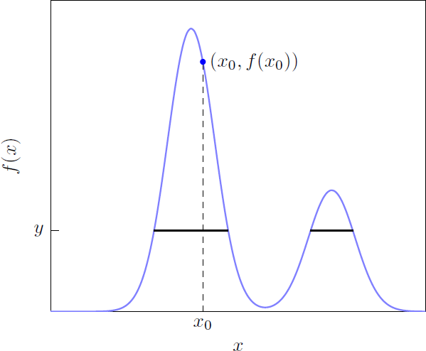
The slice sampler is motivated by the fact that sampling from $f_{\text{Δ}}\left(Z\right)$ is equivalent to sampling uniformly from the region under the density function. The ‘simple’ slice sampler constructs a Markov chain that converges to this uniform distribution by alternating between two steps: 1) sample y uniformly from the interval $\left[0,f_{\text{Δ}}\left(Z_k\right)\right]$ given some predetermined Z_k; and 2) sample Z_k+1 uniformly from the ‘slice’ $\mathcal{S}\left(y\right)=\left\{Z:f_{\text{Δ}}\left(Z\right)>y\right\}$.^[11] Iterating over this process generates a sequence of dependent draws from the target density. Figure 2 illustrates this idea in a univariate setting.

Mira and Tierney (2002) prove that if the target density is bounded and has support with finite Lebesgue measure, then the simple slice sampler is uniformly ergodic. More importantly, as noted by Roberts and Rosenthal (1999), the simple slice sampler is almost always geometrically ergodic, which is a property shared by very few other MCMC algorithms. These properties have led to slice sampling becoming a widely used method for sampling from non-standard distributions in low dimensions, although the applicability of the simple slice sampler is limited. In the multivariate setting, sampling uniformly from $\mathcal{S}\left(y\right)$ is generally infeasible, making the second step of the simple slice sampling algorithm impractical. To address this, the second step is typically modified to sample a Markov chain on $\mathcal{S}\left(y\right)$, which maintains the uniform distribution over the slice as its invariant distribution.

In the multivariate setting, the slice sampler can be implemented by updating each variable in turn or all variables simultaneously. We build on Matlab's implementation of the slice sampler, which updates all variables simultaneously.^[12] Sampling directly from a uniform distribution over the slice is infeasible in the current setting. However, as discussed above, any update that leaves the uniform distribution over the slice invariant will yield a Markov chain that converges to the target distribution. Matlab's implementation of the slice sampler updates the chain in a way that satisfies this condition using an approach described in Neal (2003). To briefly summarise, this procedure involves: randomly positioning a hypercube with side width w around the initial point; drawing a point from a uniform distribution over the hypercube; and repeatedly shrinking the hypercube (‘shrinking in’) if the candidate draw lies outside the slice until a draw is obtained within the slice.

To give an example of the shrinking-in procedure, consider the univariate setting illustrated in Figure 2. Let [x_l, x_r] be an interval of width w randomly positioned around x₀. Consider a random draw x^(p) from the uniform distribution over [x_l, x_r]. If $x^{\left(p\right)}\in \mathcal{S}\left(y\right)$, we set x₁ = x^(p). If $x^{\left(p\right)}\notin \mathcal{S}\left(y\right)$, we shrink the interval by setting x_l = x^(p) if x^(p) < x₀ or x_r = x^(p) if x^(p) > x₀. We draw again from the uniform distribution over the updated interval, repeating this process until we obtain a draw within $\mathcal{S}\left(y\right)$.

The choice of w will affect the speed at which the Markov chain converges to the target distribution and the sampler's computational efficiency. Under the general class of identifying restrictions we consider, there is no guarantee that $𝒬\left(\varphi |S\right)$ is path connected, which means the smoothed density $f_{\text{Δ}}\left(Z\right)$ may be multimodal. A small value of w may lead to difficulties moving between modes and slow convergence. On the other hand, setting w too large can make the sampler computationally inefficient, because many shrinking-in steps may be required to obtain a draw that lies within the slice. We try to balance these considerations by using a ‘contaminated’ proposal, where w = 1 with 95 per cent probability and w = 3 with 5 per cent probability. Choices of w on this scale seem reasonable given that, for small values of ∆, the target distribution resembles a truncated multivariate standard normal distribution.

Footnotes

This step could be modified to impose an alternative sign normalisation (e.g. diag$\left(A_0^{-1}\right)\ge 0_{n\times 1}$). [10]

It is only necessary to evaluate $f_{\text{Δ}}\left(Z\right)$ up to a constant of proportionality. [11]

As discussed in Neal (2003), extensions of the slice sampler can make use of local information about the shape of the target density, such as by using local quadratic approximations based on the derivatives of the log target density. The regularised constraints that we use allow us in principle to construct such approximations. Further work could potentially improve the efficiency of our approach by using this information. [12]