RDP 2025-03: Fast Posterior Sampling in Tightly Identified SVARs Using ‘Soft’ Sign Restrictions Appendix B: Additional Empirical Results
May 2025
- Download the Paper 1.45MB
B.1 Oil market shocks
B.1.1 Approximating identified sets
According to the upper bound in Theorem 3 of Montiel Olea and Nesbit (2021), the number of draws M required from inside the identified set to guarantee a misclassification error less than occurs with probability at least is , , where d is the dimension of the parameter region being approximated (i.e. the number of impulse responses). Setting d = 3 × 3 × 21 = 189 and yields M = 20,713.
This many draws is also consistent with other combinations of and . Following the recommendation in Montiel Olea and Nesbit (2021), Figure B1 plots the ‘iso-draw curve’, which traces out combinations of that support the target value of M.
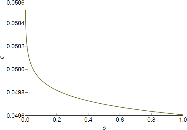
Note: Iso-draw curve plots pairs such that M = 20,713 draws from inside the identified set guarantees misclassification error less than with probability at least 1 – .
To obtain M effective draws from inside the identified set, we need to correct for the fact that the effective sample size is not 100 per cent (since some draws from the smoothed target density will violate the restrictions). We therefore gross up M using the average effective sample size from the exercise in Section 5.2. In that exercise, the average ESS was 82 per cent, so obtaining approximately M effective draws on average across the draws of requires approximately draws of Q from the smoothed target density.
B.1.2 Prior informativeness
Section 5.3.1 qualitatively discusses the role of the conditional prior for Q in driving posterior inferences about the effects of oil market shocks by comparing the results obtained under the standard and robust Bayesian approaches to inference. Giacomini and Kitagawa (2021a) suggest quantifying the influence of the conditional prior in driving posterior inferences using the ‘prior informativeness statistic’. This is the amount by which the selection of a single conditional prior narrows the credible intervals relative to the robust credible intervals:
When the parameter of interest is point identified, the credible and robust credible intervals coincide, the conditional prior has no influence on posterior inference, and the prior informativeness statistic is zero. Larger values indicate that the conditional prior contributes an increasing proportion of the information contained in the posterior.
We compute this statistic for the impulse response of each variable to each shock at each horizon, then average it over horizons (Table B1). Consistent with the discussion in Section 5.3.1, the prior informativeness statistic tends to be smaller for the responses to an oil supply shock than for the responses to other shocks. This indicates that the responses to an oil supply shock are more tightly identified, so the conditional prior contributes less of the apparent information in the posterior. The prior informativeness statistic averages less than 0.3 for all impulse responses, suggesting that the bulk of the information in the posterior is contributed by the data (given the identifying restrictions) rather than the conditional prior.
| Variable | Shock | ||
|---|---|---|---|
| Demand | Oil-specific | Supply | |
| Activity | 0.09 | 0.30 | 0.10 |
| Production | 0.20 | 0.23 | 0.06 |
| Price | 0.25 | 0.30 | 0.16 |
| Notes: Average of prior informativeness statistic over horizons. Higher values indicate that conditional prior has greater influence on posterior. | |||
B.1.3 Informativeness of identifying restrictions
Section 5.3.2 qualitatively assesses the identifying power of the narrative restrictions in the oil market model by comparing sets of posterior medians obtained under different identifying restrictions. The identifying power of restrictions can be quantified using a measure from Giacomini and Kitagawa (2021a). Let Ms be a model imposing a set of identifying restrictions and M1 be a model that relaxes the restrictions. For a given impulse response , the identifying power of the restrictions imposed in Ms beyond those imposed in M1 can be measured by:
This measures by how much the restrictions in Ms shrink the set of posterior medians compared with M1. If the additional restrictions in Ms are point identifying, the informativeness measure is one (because the set of posterior medians has zero width), while smaller values represent less additional identifying power in Ms relative to M1. Setting M1 as the ‘baseline’ model that imposes the sign and elasticity restrictions only, we compute the informativeness statistic for the two sets of narrative restrictions. For each variable and shock, Table B2 presents the average of the informativeness statistic over horizons.
| Variable | Shock | ||||||
|---|---|---|---|---|---|---|---|
| August 1990 | Full set of restrictions | ||||||
| Demand | Oil-specific | Supply | Demand | Oil-specific | Supply | ||
| Activity | 0.92 | 0.71 | 0.39 | 0.93 | 0.76 | 0.51 | |
| Production | 0.68 | 0.59 | 0.21 | 0.72 | 0.67 | 0.40 | |
| Price | 0.62 | 0.83 | 0.25 | 0.70 | 0.87 | 0.41 | |
| Notes: Average of informativeness of restrictions statistic over horizons. Informativeness is measured relative to ‘baseline’ model that imposes sign and elasticity restrictions only. Higher numbers indicate ‘more informative’ restrictions. | |||||||
The statistic obtained under the full set of restrictions is larger than when imposing the restriction based only on the August 1990 episode, since adding restrictions must (weakly) sharpen identification. But, consistent with the discussion in Section 5.3.2, the informativeness statistics under the two sets of narrative restrictions tend to be quite close. This implies that much of the identifying power in the full set of narrative restrictions is attributable to the restriction on the August 1990 episode.
B.2 Additional application: US monetary policy
To explore whether the favourable performance of our approach persists in a larger model, we use the monetary SVAR from Antolín-Díaz and Rubio-Ramírez (2018). They estimate the effects of monetary policy on the US economy using a six-variable SVAR in which the monetary policy shock is identified using an extensive set of sign restrictions on impulse responses and narrative restrictions.[27]
The reduced-form VAR is the same as in Uhlig (2005). The endogenous variables are real GDP (GDPt), the GDP deflator (GDPDEFt), a commodity price index (COMt), total reserves (TRt), non-borrowed reserves (NBRt) (all in natural logarithms) and the federal funds rate (FFRt); see Arias et al (2019) for details on the variables. The data are monthly and run from January 1965 to November 2007. The VAR includes a constant and 12 lags.
The sign restrictions on impulse responses to a monetary policy shock follow Uhlig (2005). The response of FFRt+h is non-negative for h = 0,1,...,5 and the responses of GDPDEFt+h, COMt+h and NBRt+h are non-positive for h = 0,1,...,5.
We impose the extended set of narrative restrictions from Antolín-Díaz and Rubio-Ramírez (2018). The restrictions are that the monetary policy shock was: positive in April 1974, October 1979, December 1988 and February 1994; negative in December 1990, October 1998, April 2001 and November 2002; and the most important contributor to the observed unexpected change in FFRt in these months. The implementation of the accept-reject sampler and our approach based on soft sign restrictions and the slice sampler is identical to that described in Section 5.2.
Obtaining the desired number of draws takes 20.1 hours using the accept-reject sampler, but only around 1.4 hours using our approach. The average effective sample size from the slice sampler is around 74 per cent, so our approach generates about 520,000 effective draws per hour, compared with about 50,000 effective draws per hour for the accept-reject sampler. Consistent with the results in Section 5.4, our approach also more accurately determines whether the identified set is non-empty; the posterior plausibility of the identifying restrictions based on our sampler is 43.6 per cent compared with only 5 per cent when using the accept-reject sampler.
Figure B2 summarises the posterior distributions of the impulse responses to a monetary policy shock obtained using the two samplers. The results are fairly similar, though the credible intervals based on the accept-reject sampler tend to be somewhat wider than those obtained using our sampler. This difference may reflect the ability of our sampler to better classify relatively small identified sets as non-empty. Overall, we conclude that our method continues to perform favourably in a larger SVAR.
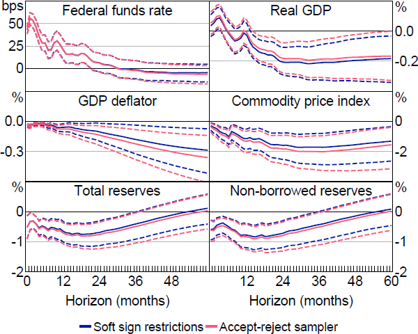
Note: Solid lines are posterior medians and dashed lines are 68 per cent credible intervals.
Footnote
See Giacomini et al (2023) for a robust Bayesian treatment of this application. [27]