RDP 2025-02: Boundedly Rational Expectations and the Optimality of Flexible Average Inflation Targeting 3. Optimal Policy – The Unconstrained Case
April 2025
- Download the Paper 1.64MB
We start with the unconstrained optimal policy problem given by Equations (9) to (13). The policymaker is free to choose any policy today and into the future that they would like. Appendix A.1 contains the full derivations for all results; here we summarise the key equations to build intuition.
Monetary policy in this case is a powerful tool even with bounded rationality because the path of interest rates is common knowledge. If the central bank only faces the demand shock, then it is able to perfectly stabilise the economy as in the standard FIRE case.
Result 1 (IS curve irrelevance). The IS curve is not a constraint when the path of interest rates is known and credible. Demand shocks (and other shocks that do not affect the gap between the efficient and flexible-price levels of output, such as productivity shocks) may be perfectly offset with current and promised changes in the interest rate, generating no welfare loss.
The trade-off for the central bank, therefore, lies with ‘cost-push’ shocks (i.e. shocks that do affect the gap between the efficient and flexible-price levels of output).
To characterise optimal policy for cost-push shocks, we take the first-order conditions with respect to and xt for the central bank's policy problem and eliminate the Lagrange multiplier on the Phillips curve:
where L is the lag operator and is the Lagrange multiplier on the updating rule for learners' inflation expectations. The term represents the benefit of increasing learners' inflation expectations and is determined by the first-order condition with respect to :
Solving Equation (15) for gives
where and and are the roots of the characteristic polynomial associated with Equation (15).[10]
Result 2 (Unconstrained optimal target criterion). The optimal target criterion is
which is composed of two distinct parts:
- a weighted-average inflation target (WAIT)
- pre-emptive policy actions based on expected future trade-offs between inflation and output gaps due to drifts in learning beliefs.
The WAIT term represents a commitment to the forward-looking rational agents. The policymaker promises to adjust the output gap in response to a weighted average of past inflation. Shocks today that generate misses in the inflation target imply future policy adjustments, lessening the equilibrium impact of any shock.
The pre-emption term represent the management of backward-looking adaptive learning expectations and is present if g > 0. The policymaker forms a belief about how inflation expectations are likely to evolve in the future given current and past misses in inflation, which are propagated through the adaptive learning component of beliefs. Drifts in inflation change the trade-off between future inflation and output gaps. Additional policy today can pre-empt future undesirable movements in this trade-off, or engineer more favourable ones.
A key feature of the optimal target criterion (17) is that it encapsulates the target criteria from a range of different primitive assumptions about how agents form beliefs as special cases. Table 1 summarises the target criterion for the special cases discussed in the previous section. Optimal policy in this case is WAIT + pre-emption. The table, however, includes a fixed belief case of = 0 and g = 0, which is of interest because it recovers the same target criterion that is implied under FIRE for discretionary policy. This case reveals that so long as expectations can be influenced, that is, g > 0 and/or > 0, it makes sense to deviate from the standard FIRE optimal discretion policy, that is, from inflation targeting.
| Case | Target criteria | Policy |
|---|---|---|
| FIRE, = 1 | = – pt | PLT |
| Hybrid NK PC, 0 < < 1, g = 1 | Equation (17) | WAIT + pre-emptive |
| Myopia/level-k, g = 0 | WAIT | |
| Adaptive learning, = 0 | IT + pre-emptive | |
| Fixed beliefs, = 0, g = 0 | IT | |
| Notes: Optimal target criteria in special cases. No terms from optimal target criteria drop out for Hybrid NK PC (New Keynesian Phillips curve) parameters. PLT stands for ‘price level targeting’; IT stands for ‘inflation targeting’. | ||
3.1 Mechanics of optimal policy
To see how policy works in practice in response to a shock, let the cost-push shock follow a first-order autoregressive process such that EtuT depends only on ut for . Recall from Equation (16) that the Lagrange multiplier on learners' inflation expectations is a function of past and current expectations of inflation at different horizons. In Appendix A.1, we show that, in the optimal equilibrium solution, this multiplier can be written
for some positive constants ax, and au. Sensibly, optimal policy aims to lower learners' inflation expectation when inflation itself is high, when their expectations are high, or when the cost-push shock is positive. This desire for lower inflation though is tempered by a desire to close the output gap, which gives rise to the positive relationship with xt. Using Equation (18), we can write the optimal target criterion (17) (in equilibrium) as
where and .
Equation (19) reveals that optimal policy adjusts the output gap in response to an exponentially weighted average of current and past inflation, , and cost-push shocks, where the weight on lag j is . In addition, relative to FIRE, the central bank increases its response to current inflation while also responding to learners' inflation expectations – pre-emption – because both affect future inflation due to drifting inflation expectations. The central bank also must respond separately to the cost-push shock ut (beyond its effect on current inflation). How aggressive or accommodative policy is with respect to past inflation, expectations, or the shock depends on and g, that is, how quickly these interventions show up in expectations.
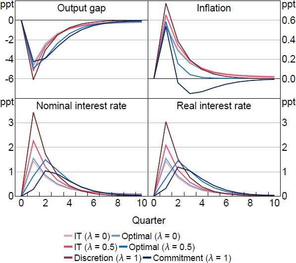
Figure 1 shows the optimal response to a cost-push shock as is varied compared to policy under an inflation-targeting (IT) regime ( and ). IT here is equivalent to the optimal targeting criteria implied under rational expectations discretion.

Notes: Response to a 1 per cent cost-push shock, which occurs in period 1. Parameter values are = 0.95, g = 0.08, = 0.99, = 1, = 0.1, /7.87.
Optimal policy for a wide range of s implies initially a muted response followed by a more aggressive policy in the medium run compared to IT. In the high cases, policy reflects the make-up quality of WAIT. Higher inflation now means a higher interest rate in the future even as inflation falls. The expectation of this policy is capitalised into current expectations blunting the impact of the shock and lessening the need to initially raise interest rates aggressively.
In the low cases, policy reflects the different way a shock propagates when there is learning. Backward-looking agents' expectations are less sensitive to the shock on impact because their expectations are anchored to the past. This means the shock has less of an impact initially, which allows for a muted interest rate response by policymakers. However, the learning process endogenously propagates the shock as expectations are revised. This leads to a growing inflation impulse over time because of rising . The optimal policy response to this growing impulse is a higher interest rate in the medium run to constrain inflation and output. The optimal policy, therefore, for a wide range in follows the same prescription: muted on impact and more aggressive over the medium run. This is true even though the rationale for why the central bank should enact such a policy changes as is varied.
Optimal policy only departs from this pattern when is close to zero. Here, the WAIT term is nearly absent and pre-emption is the dominant feature of policy. Stronger policy is required in these cases initially to blunt the propagation of the shock in beliefs. This represents the flexibility required by optimal policy in FAIT. If a policymaker expects expectations to drift, that is, become unanchored, in response to a shock, then more aggressive policy is required now.
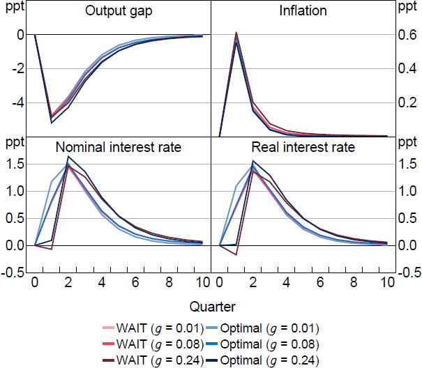
For moderate values of , however, the pre-emption motive is secondary to WAIT. Figure 2 illustrates how pre-emption affects policy when = 0.5 as we vary g making expectations more or less responsive to the shock. The figure shows WAIT ( and ) compared to optimal policy. The difference between WAIT and optimal policy is pre-emption. The WAIT policy delivers lower interest rates and real rates in each case. Pre-emption on the other hand increases the current response as g increases to counter the greater influence of the shock in causing drifts in learned expectations.

Notes: Response to a 1 per cent cost-push shock, which occurs in period 1. Parameter values are = 0.5, = 0.95, = 0.99, = 1, = 0.1, /7.87.
There are of course other scenarios where even with moderate values of pre-emption becomes more central. For example, when shocks are very persistent or the central bank expects to be constrained in the future such as when the ZLB binds, which we explore in Section 4.
3.2 The optimal average inflation target
The continued importance of WAIT relative to pre-emption shown in Figure 2 when is small is surprising. The reason it occurs is that the expectations of adaptive learners in our set-up evolve as a weighted average of current and past inflation,
Pre-emption, therefore, is an optimal response to a weighted average of past inflation. It turns out that that weighted average implied by the pre-emption component of optimal policy in equilibrium shares many features with the original WAIT component of optimal policy. In fact, it is possible to rewrite optimal policy as a simple WAIT policy with different weights that share a similar geometric decay over time.
To illustrate, substitute the weighted-average expression above for adaptive learning beliefs into the rewritten optimal target criterion (19) and rearrange:
where . The average inflation measure that a policymaker should target is a weighted average of two exponentially weighted averages of current and past inflation.
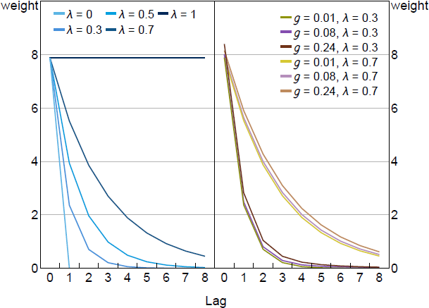
Figure 3 illustrates the similarities in the weights by plotting the term in front of from Equation (20) for different values of and g. On the left side, we plot the optimal weights for different values of when g = 0 and = 0. This calibration reflects models with myopia like Gabaix (2020) and it has no pre-emption component to policy. The high weight placed on current inflation reflects , the welfare weight on the output gap, which here is set to the welfare theoretic value of . Higher values of scale these weights profiles down while lower values raise them. When = 1, we have the optimal policy under FIRE: price level targeting. Equal weight is given to all past inflation outcomes. When = 0, there is no value to commitment and we get the rational expectations discretion outcome.
On the right side of Figure 3, we add a positive gain (g > 0) activating the pre-emption term. The optimal target criterion again responds to a weighted average of inflation. Pre-emption causes the weights to be higher depending on the specific level of g and . However, the general profile of the weights remains the same with a geometric decline over time. Optimal policy tracks a qualitatively similar weighted average of inflation when most agents have FIRE expectations and when most do not. In Section 5, we consider whether there is a single calibration for this weighted average that performs well regardless of how expectations are formed.

Notes: Plots coefficients in the power series in the first term of Equation (20), which represent the weight placed on current and lags of inflation when implementing optimal policy. Parameter values are = 0.95, = 0.99, = 0.5, = 0.1, /7.87.
In addition, it is important to note that the profiles of optimal weights are very different to the arithmetic averages that many researchers have studied when modeling average inflation targeting such as in Eo and Lie (2020) or Honkapohja and McClung (2024b). Arithmetic averages imply uniform weights over a fixed number of lags and zero thereafter. We show in Section 5 that arithmetic averages do a poor job approximating the optimal weights, while simple geometric averages approximate optimal weights well, even when the geometric weights are significantly misspecified relative to the optimal weights.
Footnote
That is, and are the solutions to the quadratic equation
For reasonable calibrations, is generally very close to and reflects the effectiveness of make-up commitments on current period inflation. The reciprocal of the explosive root reflects the persistence of the effect of current policy on future inflation (via beliefs). It is decreasing in and g, and increasing in .
[10]