RDP 2025-02: Boundedly Rational Expectations and the Optimality of Flexible Average Inflation Targeting 4. Optimal Policy – The Constrained Case
April 2025
- Download the Paper 1.64MB
We now turn to the case where the policymaker faces a constraint that prevents it from implementing a desired level of the output gap period by period. We consider two ways in which this might occur: 1) imperfect information, and 2) the zero lower bound on nominal interest rates. Again, Appendix A.2 provides detailed derivations, while we focus here on the key equations and intuition.
4.1 Imperfect central bank information
Let denote the central bank's information set in period t and let It denote the full information set. Let zT|t denote the best estimate of any variable zT conditional on , while continues to denote the expectation conditional on the full information set It. We now assume
In other words, the central bank does not possess all information in the current period necessary to implement optimal policy. The nominal interest rate it must be set each period based on incomplete information , that is,
For our purposes, it does not matter what information is missing. The key is that any missing information relevant to policy represents a constraint on current policy choices.
The optimal policy problem is to choose the sequence that maximises the welfare function (9) subject to the constraints (10) to (13) imposed by private sector equilibrium behaviour and the informational constraint (21).[11]
The first-order condition of the policymaker's problem with imperfect information with respect to it is
where is the Lagrange multiplier on the information constraint (21). Condition (22) shows that the benefit of lowering the nominal interest rate is given by the benefit of raising the output gap in the current period, and in previous periods through the fact that agents anticipate future policy responses. Condition (23) shows that the central bank should try to set the nominal interest rate so that there is no benefit to increasing or decreasing it, given the information on hand. The main difference from the unconstrained case is that demand shocks are no longer irrelevant.
Result 3 (IS curve relevance). The central bank cannot perfectly offset shocks to the IS curve when .
In the unconstrained case, when , then and so . A shock to the IS curve is irrelevant. When , the best the central bank can do is , and so and in general, which makes the IS curve a constraint on policy.
To see how this affects optimal policy, we take the expectation of (22) conditional on and using for all gives
which implies that the central bank commits to an it that balances the estimated costs of an off-target output gap in period t, , against the reduced losses in the periods before t due to expectations of . Equation (24), therefore, describes a new intertemporal trade-off, where the central bank cannot set the desired interest rate it would like, ex post, while considering ex ante how its corrections for any errors it makes interact with private sector expectations.
Taking the first-order conditions with respect to and xt, eliminating the Lagrange multiplier on the Phillips curve, and substituting in from (22) gives
which generalises Equation (14).
The information constraint implies three additional terms. The new term in on the left-hand side is zero in expectation and represents the extent to which a shock causes the central bank to ‘miss’ its intended target for the output gap. The first new term on the right-hand side – in – is an additional commitment requirement of optimal policy. It indicates how the central bank should respond to past misses caused by unexpected shocks, that is, additional make-up policy. The commitment to respond to misses in the future shifts current expectations, thereby dampening the costs of the shock. In this way, commitment under imperfect information acts as a kind of ‘automatic stabiliser’. Finally, the Lagrange multipliers on learners' inflation and output gap expectations are now
The new components in these expressions, that is, the terms in , dampen the extent of optimal make-up policy, by accounting for its effect on learners' future expectations.
Substituting the Lagrange multipliers (26) and (27) into (25), we can derive the optimal target criterion under information constraints.
Result 4 (Information constrained optimal target criterion). Recall from Equation (17) that the optimal target criterion under full information is , where is defined as
Then the optimal target criterion under imperfect central bank information is
with and
The optimal target criterion under imperfect information (28) generalises the unconstrained target criterion (17). It differs from (17) in two ways: (i) the central bank does its best to implement it given its information set (i.e. it can only control , not ), and (ii) its target for is not always zero, but adjusts based on past errors in implementing optimal policy – – due to the information constraint.
The optimal target criterion though remains a flexible average inflation target. The difference here is in the definition of flexibility. The central bank still retains the same WAIT and pre-emption incentives but now must commit to make up for any errors in implementing policy that arise from the information constraint.
Make-up policy works through three channels represented by the three terms in the first line of Equation (29). The first term reflects the effect on inflation expectations of a commitment to make up for an error. Rational forward-looking agents respond today to the expected make-up policy they anticipate will occur, which dampens the impact of the shock. The second term represents the effect of this commitment on output gap expectations, which affect the current output gap through the permanent income hypothesis with (1 – ) representing the marginal propensity to consume from a change in current period income. The final term represents the effect of commitment on nominal interest rate expectations. Committing to offset misses shifts the expected nominal yield curve and further ameliorates the effect of any unexpected shock. The first two terms are both multiplied by , which signifies their dependence on forward-looking expectations. By contrast, the third term is multiplied by one since all agents incorporate the optimal path of interest rates into their beliefs.
The second line of Equation (29) reflects the change in the cost and benefit to make-up policy when there are learning expectations. Policy actions, like shocks, are instantiated into learning agents' beliefs when output and inflation respond and must be accounted for when implementing policy. To aid intuition, consider the case when prices are fixed, = 0. The optimal target criterion reduces to
where is
with . The central bank should set its best estimate of the output gap equal to the moving target , which is determined by the previous period's miss, . The extent to which the central bank should commit to offset past misses depends on the strength of: (i) the forward-looking income expectations channel, given by ; (ii) the nominal yield curve channel, given by the 1 in the parentheses; and (iii) the effect of learners' drifting income expectations, given by . This last term lowers the response to a given miss as g rises or falls. Make-up policy itself is a source of variation in this economy when agents are learning, which generates further drifts in beliefs that must be pre-empted.[12]
4.1.1 Mechanics of optimal policy: imperfect information
Figure 4 shows how optimal policy compares with IT in response to an unexpected cost-push shock under the same calibration explored in Figure 1. In contrast to the unconstrained case, the optimal policy is now more aggressive than IT policy. IT policy ‘lets bygones be bygones’ and does not respond to the failure to recognise the shock on impact, whereas optimal policy seeks to ‘make up’ for this miss. The anticipation of the aggressive policy acts as an automatic stabiliser when the shock occurs. Forward-looking agents understand the aggressive response is coming and that inflation will be lower in the future, which lowers inflation today. When is high, optimal policy is only a little different from the unconstrained case. This is because even under perfect information, optimal policy required only a small contemporaneous response, with a larger and persistent subsequent response. The information friction is therefore not too costly and only a small increase in make-up policy is required. When is low, the information friction makes more of a difference. With perfect information, the required contemporaneous response was large and the role of make-up policy was smaller. Imperfect information prevents the contemporaneous response, but introduces a substantial role for make-up policy because policymakers now want to influence interest rate expectations, which are forward looking even when = 0. The optimal policy prescription therefore ends up being similar across in the imperfect information case.
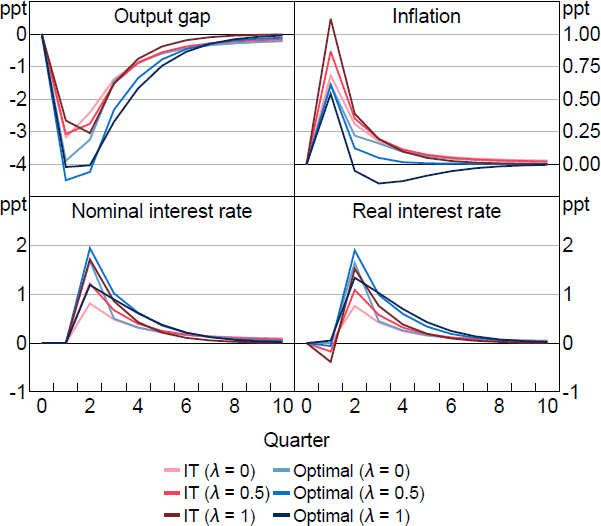
Notes: Response to a 1 per cent cost-push shock, which occurs in period 1. Parameter values are = 0.95, g = 0.08, = 0.99, = 1, = 0.1, /7.87.
Figure 5 shows the dynamics of optimal policy versus IT for an unexpected demand shock (i.e. an increase in the natural rate ). In the full information case, this shock is perfectly offset and has no effect on the output gap or inflation. Information frictions, however, change the prediction. Demand shocks generate inflation. As in the cost-push shock case, optimal policy is now more aggressive than required under IT, which causes inflation to undershoot following the shock. Once again, under imperfect information, optimal policy is similar for both high and low cases.
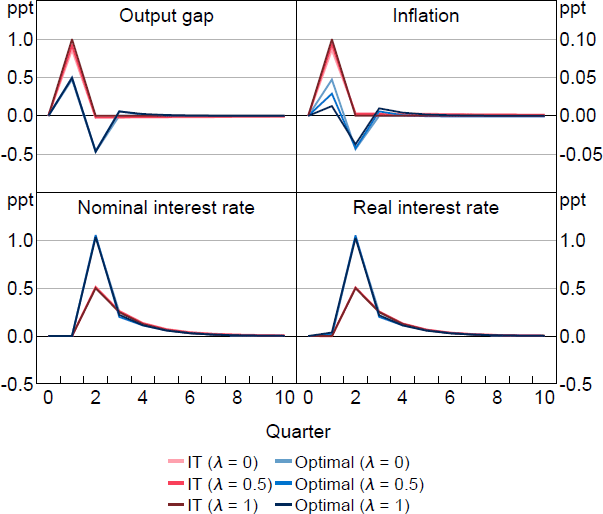
Notes: Response to a 1 per cent natural interest rate shock, which occurs in period 1. Parameter values are = 0.95, g = 0.08, = 0.99, = 1, = 0.1, /7.87.
4.1.2 Optimal average inflation target: imperfect information
Like the unconstrained case, a FAIT policy is robust because we can capture most of WAIT, preemption and the additional make-up policy using only a weighted average of past outcomes. In contrast to the unconstrained case, though, optimal policy requires tracking a weighted average over both inflation and the output gap.
To illustrate, we substitute into Equation (29), rearrange, and then substitute the result into Equation (28) to arrive at
where denotes the expectation conditional on . This formulation makes clear that the ‘moving target’ described in Equations (28) and (29) is equivalent to trying to set some weighted average of current and past equal to zero. Since the central bank cannot implement the full information optimal target criterion in every period, it instead tries to implement it on average over time.
As in the full information case, we can combine the optimal policy conditions with the equilibrium conditions to evaluate the expectation terms in Equation (30) (which are inside ). This gives us a description of optimal policy just in terms of past inflation and output gaps, akin to Equation (20). Assuming again that the cost-push is a first-order autoregressive process,[13] Appendix A.2 shows that, following an analogous approach to the derivation of Equation (20), we can write optimal policy under imperfect information in equilibrium as
where and are power series in L and are defined in Appendix A.2. The coefficients in the power series Qx and give the precise weight that the central bank places on current and past values of the output gap and inflation when implementing optimal policy.
Figure 6 plots these weights for different values of and g. The top row mirrors the left panel of Figure 3. It shows the case where there is no updating of learning beliefs (g = 0), which reduces the model to one featuring myopia as in Gabaix (2020). Optimal policy requires increasing weights in this case. This reflects the requirement of additional make-up policy. The bottom row of the figure shows the g 0 case. Additional make-up policy is required but it is moderated by the need to adjust for drifts in expectations. Importantly, when g is high, the optimal weights eventually decline in a similar way to the unconstrained case. It is this declining feature of the weights that makes FAIT a robust framework across a wide range of scenarios. We show in Section 5 that tracking weighted averages of inflation and output with declining weights captures most of the benefits of optimal policy.
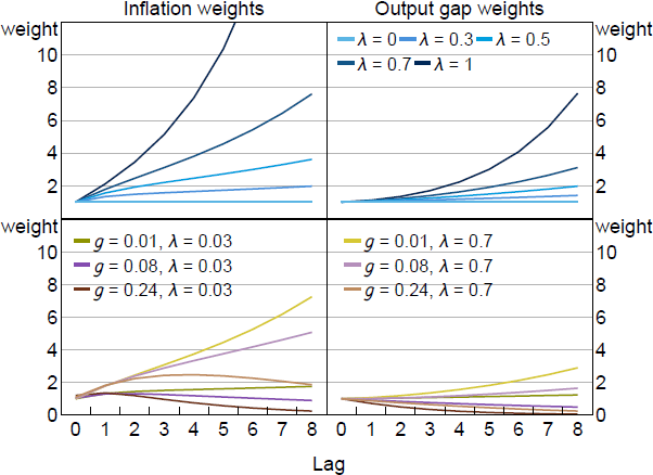
Notes: Optimal weights on past inflation and output gap under imperfect information found in and Qx (L) in (31). Parameter values are = 0.99, = 1, = 0.1, /7.87.
4.2 Optimal policy with the zero lower bound
Optimal policy with the zero lower bound is very similar to optimal policy under imperfect information. Both constraints mean that the central bank sometimes cannot set the output gap it wants, in which case it cannot implement the full information optimal target criterion. As with imperfect information, the central bank should respond to this ZLB constraint by using commitment to influence the forward-looking expectations that enter the IS equation – that is, households' expectations over future output, inflation, and nominal interest rates. The key difference from the imperfect information case is that losses caused by a binding ZLB are not zero in expectation, even in the presence of mean zero shocks drawn from a symmetric distribution. Therefore, the pre-emptive channel of policy has a more significant role. The central bank should seek to pre-emptively raise learners' output and inflation expectations if it expects the ZLB to bind in the future. This is the use it or lose it character of optimal policy when confronted with the ZLB. It is optimal to move expectations pre-emptively before the constraint binds.
To derive optimal policy with the ZLB, we replace the information constraint (21) with the lower bound constraint
The optimal policy problem is then to choose the sequence that maximises welfare (9) subject to the constraints (10) to (13) imposed by private-sector equilibrium behaviour and the lower bound constraint (32).
The first-order conditions are the same as in the imperfect information case, except that Equation (23) is replaced with the complementary slackness condition
Just as previously represented the extent to which imperfect information constrained the central bank, it now represents the losses caused by the ZLB. It is positive when the ZLB is binding and zero otherwise.
Condition (25) is the same as before, but the expressions for and in conditions (26) and (27) take a more general form, because is no longer necessarily equal to zero for all :
If for all , then conditions (34) and (35) collapse to conditions (26) and (27). The second line of (34) indicates how the central bank can use learners' inflation expectations to lower the real interest rate when the ZLB binds. The first term in the parentheses represents the effect of raising learners' inflation expectations on the inflation expectations of the rational forward-looking agents. This term, therefore, has both pre-emptive and history-dependent aspects. The second term in the parentheses represents the effect of shifting learners' inflation expectations on future real interest rates. Similarly, (35) represents the effect of shifting learners' output expectations for future output gaps.
Conditions (25), (33), (34) and (35) define optimal policy with the ZLB constraint.
Result 5 (Optimal target criterion with ZLB). Recall that the optimal target criterion under full information and without the ZLB is , where we defined
Then the optimal target criterion when the ZLB can bind is
where and
where
is the same as Equation (29) and
Optimal policy commits to responding to past misses (see P(L)), exactly as in the information constraint case, and it adjusts the target in response to expected future target misses (P1(L–1)) and past expectations of target misses (P2(L) and P3(L–1)). The net effect is even more make-up policy is promised.
The terms P1(Z–1) and P3(L–1) capture the insurance nature of optimal policy when agents are learning. Eusepi, Gibbs and Preston (2024) coin the term the insurance principle, which says that when the duration of the ZLB is uncertain, and agents are learning, that larger front-loaded forward guidance promises are optimal. These policies are too stimulatory when the shock is short-lived, but highly effective when the shock is long-lived because of the positive contribution they make to agents' drifting beliefs. The expectations operator present in these two terms captures the idea that policy must be set according to the expectation of how long the ZLB binds, which may not match the ex post realised duration of the shock. The more learning that is present (lower ), and the faster learning happens (higher g), the more the central bank should respond now to these expectations of future binds of the ZLB.
To more clearly see how the terms in Result 5 relate to make-up and insurance policies, consider again the case where prices are fixed, . Optimal policy implies
where
with . The first line is identical to the target criterion in the imperfect information case with fixed prices. The second line represents the additional requirement of optimal policy to lift agents' expectations pre-emptively when the ZLB is expected to bind, or continue to bind. Policy should move in anticipation of a binding of the ZLB to raise expectations to pre-empt the losses that are expected to accrue while the ZLB binds.
Figure 7 compares optimal policy to IT in the presence of the ZLB.[14] First, note that even before the shock hits, optimal policy maintains a small positive output gap and inflation rate (except when g is very small). This is the pre-emptive component of optimal policy: given that the ZLB could bind with some probability in any period, it is optimal to ensure that learners' inflation and output gap expectations are somewhat above target. For larger g, shocks have greater influence over learners' expectations, and so it is optimal to ‘run the economy hotter’. Optimal policy also holds the policy rate at the ZLB for longer than IT, generating a positive output gap and inflation overshoot. This is the make-up component. As a result of these two components, the downturn when the shock hits is much smaller, even though there is some welfare loss before and after the shock. Interestingly, even though optimal policy involves a more expansionary stochastic steady state, the policy rate is higher, because inflation expectations are higher.
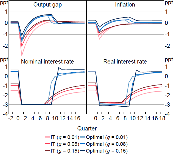
Notes: Response to a 1.5 per cent natural rate shock, which occurs in period 1 and has persistence 0.75. Parameter values are = 0.25, = 0.95, = 1, = 0.1, /7.87.
Figure 8 shows how the pre-emptively higher stochastic steady-state inflation target varies with , g, and the mean neutral rate, rn.[15] As expected, the inflation target is higher when g is higher, which requires more pre-emptive policy, and when rn is lower, which increases the likelihood of hitting the ZLB. When g is high, the inflation target is highest for intermediate values of , reflecting the amplification that can occur between forward-looking and backward-looking expectations through optimal pre-emptive policy.
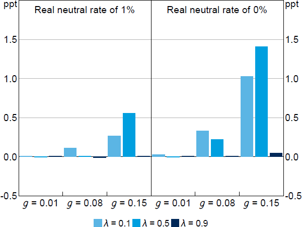
Notes: We assume that the deterministic inflation steady state is 2 per cent, so, for example, rn = 1% implies that the ZLB is 3 percentage points below steady state. The standard deviation of is 4 percentage points. Parameter values are = 0.95, = 1, = 0.1, /7.87.
Footnotes
The private sector continues to make decisions based on the full information set, It. This means that when an unexpected shocks occurs, their expectations of future policy will adjust before the central bank moves the actual policy rate. This is what underlies the ‘automatic stabiliser’ mechanism discussed below. [11]
Eusepi, Giannoni and Preston (2024) explore this feature of learning models in depth, focusing on the transmission of short-run interest rate to long-run interest rate expectations, which is absent in our model. In Appendix B.1, we discuss how our results might be affected if some agents form policy rate expectations by learning, instead of rationally. [12]
Only the unexpected component of the IS curve shock is relevant to optimal policy. The central bank can fully offset any expected component, just as it does in the full information case. [13]
To solve the model with the ZLB, we use a policy function iteration method, drawing on code in Sijmen Duineveld's PROMES toolbox (Duineveld 2021). [14]
Here, when we say ‘steady-state inflation target’, we are referring to the stochastic steady state, meaning the value that inflation converges to in the absence of shocks, but where agents still expect that shocks could occur in the future. [15]