RDP 2025-02: Boundedly Rational Expectations and the Optimality of Flexible Average Inflation Targeting 5. Comparing Target Criteria
April 2025
- Download the Paper 1.64MB
The optimal target criteria we have derived require complex considerations on the part of the central bank where policy must respond to competing objectives in precise ways. The target criteria also requires a knowledge of the underlying expectation formation process in order to implement. In this section, we ask how robust are the policy lessons we draw from the optimal criteria. In other words, how flexible can you be as a flexible average inflation targeter?
To answer this questions, we first look at how closely simple weighted-average inflation targeting schemes can perform relative to the optimal target criteria, and how do these perform against known target criteria like inflation or price-level targeting. Second, we study how these simplified optimal target criteria perform when a central bank does not know how expectations are formed and must calibrate their target criterion to maximise the average welfare for a range of different belief formation processes.
We allow for cost-push shocks and imperfect central bank information in this analysis so the policy cannot perfectly offset all demand and productivity shocks. We consider this to be the most general and realistic case.[16] Appendices D.1 and D.2 provide results for the unconstrained case, where cost-push shocks are the only source of losses.[17]
5.1 Approximating optimal policy with simple target criteria
Table 2 presents a list of simple target criteria that capture key features of the optimal target criteria in the unconstrained and constrained cases, as well as other target criteria commonly studied in the literature. The list includes inflation targeting, price-level targeting, and simple average inflation targeting rules (‘k-yr AIT’). Informed by the analytical results in the previous sections, we also include rules that incorporate some combination of an IT or weighted AIT component (‘WAIT’); a weighted average output-gap targeting component (‘WAXT’); and a preemptive component that is a forward-looking weighted average of inflation forecasts (‘preemptive’).
| Rule | Form | Parameters |
|---|---|---|
| IT | ||
| PLT | ||
| k-yr AIT | ||
| WAIT | ||
| WAIT + WAXT | ||
| IT + pre-emptive | ||
| WAIT + pre-emptive | ||
| WAIT + WAXT + pre-emptive | ||
| Note: The parameters are optimised to minimise welfare loss when implementing each rule. | ||
For each of the target criteria listed in Table 2, we find the optimal parameters that minimise welfare loss and compare it to the loss achieved under the fully optimal target criteria. For the calibration, we set = 1 and = 0.1 (equivalent to a Calvo stickiness probability of around 0.7). For the expectation formation parameters, we use a baseline of = 0.5, g = 0.08 and = 0.95. Finally, we set the persistence of the shocks to = 0.5 with the standard deviation of the neutral rate shock at ten times the standard deviation of the cost-push shock (similar to Giannoni (2014)). For simplicity, we let , so that the loss function is , with /7.87.
Table 3 presents the results. The gains from optimal policy relative to IT are large, at 36.5 per cent of the loss under IT. These gains can be almost entirely achieved by following a rule that responds to a weighted average of both past inflation and past output gaps (the ‘WAIT + WAXT’ rule). Significant gains come from making up for past output gaps, because imperfect information prevents the central bank from perfectly controlling the output gap. Recall that lagged output gap terms enter the optimal target criterion under imperfect information, Equation (28) (as with the ZLB), unlike the unconstrained case, Equation (17). The decay parameters in the WAIT and WAXT are 0.94 and 0.89, so substantial weight is placed on inflation and output outcomes in the past. The PLT rule outperforms IT. Simple AIT rules with short windows perform worse than the weighted average rules.
| Rule | Loss (% relative to IT) | |||||
|---|---|---|---|---|---|---|
| 5-yr AIT | 24.6 | 27.4 | ||||
| IT | 0 | 20.9 | ||||
| 2-yr AIT | −4.5 | 27.9 | ||||
| IT + pre-emptive | −14.8 | 0.0 | 1.60 | 1.75 | ||
| 1-yr AIT | −15.7 | 15.6 | ||||
| PLT | −23.8 | 20.3 | 1 | |||
| WAIT | −25.1 | 17.4 | 0.75 | |||
| WAIT + pre-emptive | −25.1 | 17.4 | 0.75 | 0.00 | undef | |
| WAIT + WAXT | −35.4 | 12.3 | 0.94 | 0.89 | ||
| WAIT + WAXT + pre-emptive | −35.4 | 12.3 | 0.94 | 0.89 | 0.00 | undef |
| Optimal | −36.5 | |||||
| Notes: Welfare losses are normalised relative to the welfare under IT. The parameters for each rule are optimised to minimise welfare. The optimal value of a parameter is undefined (labelled undef) if the parameter has no effect on loss at the optimum. | ||||||
The results support the idea that the average in FAIT should be a weighted average. Importantly, though, the simple target criteria all require a strong response to current inflation, which is seen by the optimised values of and . Simple AIT rules require large values as well to compensate for the 1/k weight applied to current inflation. However, it is not enough to offset the wrong type of average.
5.2 Robust optimal policy under parameter uncertainty
The previous results show that simpler targeting rules can approximate the optimal target criteria. However, the simple targeting rules require the policymaker to know , g and . Here we study what happens when the policymaker does not know these values and instead must choose a target criterion that is optimised to maximise welfare on average when , g and can take on any value in economically meaningful ranges, which we approximate with a grid. In particular, we consider the values: {0,0.25,0.5,0.75,1}, g {0,0.01,0.08,0.25,1} and p {0.95,0.99}.[18]
Table 4 shows the average welfare and the optimised parameter values for each target criterion. In addition, we show the average loss that would be achieved if the optimal criterion was implemented at each point of the grid, which represent the minimum loss achievable. WAIT rules perform best, with decay parameters of around 0.75 to 0.87. Making up for past output gaps as well via a WAXT component substantially lowers the loss. The PLT rule significantly outperforms IT. The 5-yr and 2-yr AIT rules always perform poorly.
| Rule | Average loss (% relative to IT) | |||||
|---|---|---|---|---|---|---|
| 5-yr AIT | 118.0 | 1.4 | ||||
| 2-yr AIT | 19.8 | 9.2 | ||||
| IT | 0 | 20.9 | ||||
| IT + pre-emptive | −1.3 | 14.9 | 13.0 | 1.52 | ||
| 1-yr AIT | −16.6 | 20.7 | ||||
| PLT | −22.4 | 16.8 | 1 | |||
| WAIT | −24.0 | 15.1 | 0.75 | |||
| WAIT + pre-emptive | −24.0 | 15.1 | 0.75 | 0.0 | undef | |
| WAIT + WAXT | −31.0 | 14.5 | 0.87 | 0.69 | ||
| WAIT + WAXT + pre-emptive | −31.1 | 13.3 | 0.87 | 0.66 | 6.8 | 0.00 |
| Optimal | −35.7 | |||||
| Notes: The parameters reported are set to maximise the average loss across all points in the grid. Average welfare losses are normalised relative to the welfare under IT. The optimal value of a parameter is undefined (labelled undef) if the parameter has no effect on loss at the optimum. | ||||||
To show what lies behind the average losses in the table, Figure 9 plots the loss under a selection of target criteria from Table 4 for different values of the expectation formation parameters and g. The parameters in the policy rules are held fixed at the robustly optimal values set to minimise average loss and not optimised for each and g shown in the figure. The dashed line shows the optimal target criteria optimised at each point to show how close the simple rules with the average coefficients can come to the fully optimal policy.
The results in Figure 9 reflect the nesting of different expectations assumptions within our approach. The IT rule and PLT rules perform similarly when is low (when make-up commitments have little effect on inflation or output gap expectations) or g is high (when the sensitivity of learners' beliefs increases the cost of make-up commitments relative to their benefit).[19] When is high, make-up commitments are more powerful and the IT rule performs poorly.
In contrast, the WAIT rules generally perform well for all and g, and including a WAXT component consistently lowers the loss for all parameters (except for g = 1, when it has little effect). It is important to reiterate that this is the case even though we have fixed the coefficients of the simple WAIT and WAXT rules to their robustly optimal values in Table 4 so it is a fair comparison with the IT and PLT rules. Only in the optimal policy benchmark do we allow the policy rule parameters to change as we vary and g. The performance of the fixed-coefficient simple WAIT and WAXT rules is still remarkably close to the optimal benchmark, which illustrates the robustness of this form of FAIT.
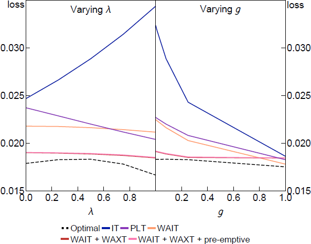
Notes: The parameters in the policy rules are fixed at the robustly optimal values presented in Table 4. For the other parameters (other than the one changing), we set = 0.5, g = 0.08, = 0.95, = 0.1, = 1, = 0.5, = 1 and = 0.1.
5.3 Discussion
The reason that simple FAIT target criteria are robust is that once and g are in the interior of their theoretical ranges, and expectations are both backward looking and forward looking, the features of optimal policy are the same. Optimal policy requires a weighted-average inflation target and some flexible component that captures pre-emption and make up. Pre-emption appears to be satisfied in most cases simply by placing high weight on current inflation and output realisations as found in the optimised and coefficients in the WAIT + WAXT rules, while additional make-up policy is captured by including the WAXT term.[20]
Footnotes
Alternatively, we could also allow for an occasionally-binding ZLB. However, as we show in Result 5, imperfect central bank information captures key features of the ZLB constraint, in that both prevent the central bank from perfectly controlling the output gap. The main difference is that target misses due to the ZLB are non-zero in expectation, so allowing the ZLB when optimising the simple target criteria outlined below would likely result in a stronger pre-emptive response to expected future outcomes. [16]
The main difference is that the optimal degree of make-up policy is lower when the central bank has perfect control of the output gap, as the analytical results in previous sections suggest. Compared to the imperfect information case, the optimal weight on lagged inflation and output gap outcomes is smaller, PLT underperforms IT, and IT in general is closer to optimal policy. That said, Appendix C.2 shows that allowing for an infinite-horizon Phillips curve somewhat increases the optimal degree of make-up policy in the unconstrained case, making it more like the imperfect information case. [17]
We set the other parameters at the baseline calibration described in the previous section. [18]
PLT still slightly outperforms IT even when = 0 because nominal interest rate expectations still respond to make-up commitments. If the central bank has perfect control of the output gap, then IT outperforms PLT significantly when = 0 (see Appendix D.2). [19]
If we allowed for the ZLB, including an explicit pre-emption term would likely offer a greater improvement in welfare (at least if the steady-state neutral rate is sufficiently low). Increasing the persistence of the cost-push shocks might have a similar effect. [20]