Research Discussion Paper – RDP 2022-01 MARTIN Gets a Bank Account: Adding a Banking Sector to the RBA's Macroeconometric Model
1. Introduction
Despite the real economy and banking system being inextricably intertwined, within the Reserve Bank of Australia (RBA) they are currently modelled separately. In the RBA's macroeconometric model, known as MARTIN (Ballantyne et al 2019), the difference between banks' mortgage rates and the RBA's cash rate is treated as exogenous (i.e. determined outside the model). This means that economic downturns in the model do not feed back into the banking system and change the interest rates banks charge borrowers or the amount they are willing to lend (i.e. there is no feedback to ‘credit supply’). Analogously, the RBA's bank stress testing model treats the macroeconomic scenario as exogenous, and therefore does not consider the effect a stressed banking system may have on the macroeconomy (RBA 2017).
In MARTIN, treating the banking system as exogenous does not typically lead to large model inaccuracies. This is because the interest rates banks charge borrowers ensure they are sufficiently profitable to weather most downturns without a deterioration in their capital levels. However, when faced with large downturns – such as what some countries experienced during the global financial crisis or what was feared could result from COVID-19 – loan losses may eat into banks' capital, and they may respond by increasing their loan interest rates and/or reducing the amount they are willing to lend. This response from banks amplifies the downturn – higher interest rates and reduced lending lead to lower housing prices, lower business investment and lower consumption, thereby leading to higher unemployment and a further increase in loan losses – leading to an amplified response from banks and even further amplification of the downturn. This amplification cycle is known as a ‘financial accelerator’ mechanism.
While the existence of financial accelerator mechanisms was known before the global financial crisis (Kiyotaki and Moore 1997; Bernanke, Gertler and Gilchrist 1999), it was this crisis that highlighted the failure of modern macroeconomics to fully appreciate their size and likelihood of occurring (Lindé, Smets and Wouters 2016; Gertler and Gilchrist 2018). So it is important for the RBA to have a modelling framework that incorporates at least some of these accelerator channels. Unfortunately, the best way to incorporate these channels is not obvious, as the literature has advanced in a myriad of different directions (see Appendix A for a literature review).
To fill this gap in the RBA's modelling repertoire, we build an extension to MARTIN that incorporates one of the key financial accelerator mechanisms – a banking sector that endogenously and nonlinearly changes credit supply in response to loan losses and/or changes to their funding costs. Consistent with the way MARTIN was originally designed, our approach captures how RBA staff currently model the banking system; we achieve this by basing our extension on the existing modelling frameworks used within the RBA.
The determinants of banks' funding costs are based on the RBA's funding cost model (Davies, Naughtin and Wong 2009; Brassil, Cheshire and Muscatello 2018). The determinants of household loan losses are based on the micro-simulation model developed by Bilston, Johnson and Read (2015) and updated by Kearns, Major and Norman (2020). How banks respond to these losses is based on the RBA's bank stress testing framework (RBA 2017).
Incorporating these disparate frameworks into MARTIN, while making minimal changes to the original MARTIN design, obviously requires compromises. For example, the lack of recent financial crises in Australia prevents us from using time series data to estimate the necessary relationships (the method used in the original MARTIN design). Instead, the additional MARTIN equations are calibrated from the aforementioned RBA frameworks, microdata from the Survey of Income and Housing, and the Australian Prudential Regulation Authority's (APRA) stress testing results. We also have less modelling freedom than the aforementioned frameworks, as MARTIN already includes equations for some important relationships – the relationship between credit growth and interest rates, for example.
By combining a large and complex macroeconometric model (MARTIN) with a micro-simulation model, and nonlinear stress testing and funding costs frameworks, our approach moves beyond the existing macroeconometric frontier (see Appendix A for a literature review).
After providing a summary of the new banking sector mechanisms (Section 2) and detailing the new components (Section 3), we illustrate how this new modelling framework (henceforth, banking-augmented MARTIN or BA-MARTIN) improves our ability to model the economy and allows us to answer important policy questions that could not previously be adequately answered. Specifically, we show:
- how the inclusion of a ‘financial accelerator’ mechanism changes how large shocks are transmitted through the economy (Section 4); and
- how the pass-through of monetary policy to banks' lending rates depends on the level of interest rates and the state of the economy (Section 5).
1.1 BA-MARTIN's financial accelerator mechanism
We illustrate the financial accelerator mechanism by showing how one of the more pessimistic economic scenarios that could have resulted from COVID-19 might have affected the banking sector, and subsequently the supply of credit to the Australian economy. We do this by feeding the downside scenario from the May 2020 Statement on Monetary Policy (RBA 2020c) into BA-MARTIN and then explore how much worse predicted economic outcomes would be with the additional financial accelerator mechanism. Had this scenario eventuated – with GDP 12 per cent below pre-COVID-19 forecasts and the unemployment rate surpassing 10 per cent – we estimate that loan losses would have been sufficient to reduce banks' capital. Without additional public policy support, housing prices two years after the onset of the crisis would have fallen an additional 3 per cent and 16,000 fewer people would have been employed (a 0.1 percentage point increase in the unemployment rate).
We have received feedback that the effect on the economy from our financial accelerator mechanism seems small considering how much damage the global financial crisis did to the global economy (Guerrieri and Uhlig 2016; Bernanke 2018). But there are two important distinctions between the Australian banking sector and those overseas. First, the Australian banking sector has an ‘unquestionably strong’ capital framework (APRA 2017), tends to be highly profitable (FSRC 2018), and is lower risk than other countries' banking sectors (RBA 2012). So it can weather larger storms.
Second, the majority of assets held by Australian banks are loans that can be repriced at short notice. Most loans are variable rate, and even the fixed-rate loans tend to have rates fixed for less than three years (far less than the 30-year mortgages common in the United States). Moreover, Australian variable-rate loans are not explicitly indexed to any market rate, unlike the ‘tracker’ loans that are common in some European countries (Lea 2010). This allows Australian banks to spread the cost of unexpectedly high losses across both new and outstanding loans, which leads to a much smaller effect on economic activity than if the cost were borne by new loans only (e.g. by the banks tightening lending standards, which was a common response by US and European banks during the global financial crisis (Maddalonia and Peydró 2013; Bassett et al 2014)).
That said, BA-MARTIN has the flexibility to explore what would happen if banks restricted new loans only. In the same downside scenario, and without additional policy support, housing prices two years after the onset of the crisis would have fallen an additional 12 per cent and 59,000 fewer people would have been employed (a 0.4 percentage point increase in the unemployment rate).
To be absolutely clear, these amplified numbers are scenarios not forecasts, and are designed solely to show the quantitative importance of the financial accelerator mechanism. Forecasted amplifications would be smaller, as some combination of fiscal, monetary and regulatory policies would respond to the amplified downturn.
1.2 BA-MARTIN's state-dependent monetary policy pass-through
Pass-through is affected by the level of interest rates because deposit rates tend to have a lower bound around zero – due to the possibility of holding physical currency instead (Garner and Suthakar 2021; Hack and Nicholls 2021). With deposit rates unable to move below zero, cash rate reductions cause smaller reductions in banks' funding costs than when this lower bound does not bind.
Pass-through also changes when the banking system is stressed (i.e. when losses are sufficient to reduce banks' capital). When the banking system is stressed, further reductions in net interest income or increased loan losses will lead to further contractions in credit supply. Cash rate reductions lead to reduced net interest income but they also reduce losses, with the latter effect typically dominating during periods of stress. As a result, pass-through can be greater than 100 per cent because the cash rate cut moderates the credit supply contraction in addition to the usual reduction in banks' funding costs.
2. BA-MARTIN in a Nutshell
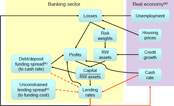
The mechanics of the new banking sector in MARTIN can be summarised as follows (see Figure 1 for a graphical representation):
- Higher unemployment, lower housing prices and higher interest rates all increase loan losses.[1]
- These loan losses directly reduce banks' profits; with sufficiently large losses causing banks' capital to fall. Losses also increase the perceived riskiness of banks' loan portfolios, so the risk weights attached to assets when determining banks' capital adequacy ratios (capital divided by risk-weighted assets) increase.
-
Australian banks hedge the majority of their interest rate risk (Brassil et al 2018). Therefore, the direct effects of interest rate changes on banks' profits can be decomposed into three components: changes in the cash rate, changes in banks' debt/deposit funding spreads and changes in the spreads between their lending rates and funding rates.
- Funding spreads are determined by offshore funding markets (as in Brassil et al (2018)), changes in credit risk (determined by changes in capital adequacy) and a zero lower bound (ZLB) for retail deposits. For a given level of lending spreads, a reduction in funding spreads or the cash rate directly reduces banks' net interest margins (NIM = net interest income divided by interest-earning assets), because banks have more interest-earning assets than interest-bearing liabilities.
- Lending spreads consist of an exogenous component (the determinants of which include competitive pressures and regulations, for example) – denoted as the ‘unconstrained lending spread’ in Figure 1 – and an endogenous response to a deterioration in capital adequacy (discussed below). A reduction in lending spreads also reduces banks' NIMs, but the effect is much larger than the effect of a funding cost change because banks have more debt than equity.
- Banks can respond to a capital deterioration in several ways; these include: raising new capital (e.g. equity issuance), reducing dividends, increasing lending spreads and reducing their willingness to lend. We assume that banks do not immediately raise new capital in response to a widespread capital deterioration.[2] Therefore, once dividend payments are minimised, banks' only remaining options for returning their capital adequacy ratios to target are to increase lending spreads and/or reduce credit growth.
-
In the baseline version of BA-MARTIN, we assume banks choose to increase lending spreads on new and outstanding loans in response to a capital deterioration.[3] We make this assumption because increasing lending spreads increases banks' NIMs, which profit-maximising banks desire.
- Prior to the capital deterioration, competition prevents banks from increasing lending spreads. The capital deterioration allows banks to increase these spreads without fear of losing market share (because there are barriers to entry and we model a deterioration that affects all banks). In other words, banks are constrained profit-maximisers whose capital constraints tighten as a result of the losses, thereby increasing their constrained profit-maximising lending spreads.
- MARTIN already has an equation that determines the relationship between lending rates and household credit growth; this equation is estimated from the historical relationship between these variables. To minimise the changes we make to MARTIN, we do not change this equation.[4] Therefore, by increasing their lending spreads (i.e. by reducing credit supply), banks increase NIMs and reduce credit growth, both of which increase their capital adequacy ratios.
- This reduction in credit supply feeds back into the real economy and amplifies losses – directly by increasing debt servicing costs and indirectly via lower housing prices and higher unemployment (i.e. the banking sector amplifies the original economic deterioration).
Notes:
Solid red arrows denote unchanged MARTIN relationships, dashed red arrows denote existing MARTIN relationships that we endogenise, and black arrows denote the new relationships. RW = Risk-weighted.
(a) Links within the real economy are excluded for simplicity.
(b) Including a zero lower bound for retail deposits.
(c) The spread banks would set if capital levels were at their desired level.
In short, we model the financial accelerator mechanism in a piecewise fashion. If losses are small and banks' capital is sufficiently high, credit growth is demand determined – that is, lending rates equal an exogenous spread over the cash rate – and the effect these losses have on the broader economy is limited to that caused by the lower shareholder returns (as is currently the case in MARTIN). Conversely, if loan losses are sufficiently large to cause banks' capital to fall below their desired level, an endogenous and nonlinear wedge forms between the actual lending spread and the exogenous spread – that is, credit supply is endogenously reduced.
Importantly, this feedback into the real economy can be offset by more expansionary monetary policy (if monetary policy is unconstrained). With this expansionary policy also leading to reduced loan losses, thereby improving capital adequacy. However, the more expansionary policy also leads to higher credit growth and a reduction in NIMs, both of which amplify the deterioration in capital adequacy. Which channels dominate will depend on the state of the economy (and is the subject of Section 5 of this paper).
How much banks reduce credit supply in response to a capital deterioration is based on the RBA's stress testing framework (RBA 2017). This framework is more complex than what could reasonably be incorporated within a macroeconometric framework. So instead of matching the stress testing framework exactly, we assume banks reduce credit supply in order to return their capital ratios to target with a speed of adjustment that broadly matches the speed of adjustment implied by the stress testing framework. This speed of adjustment is detailed in Section 3.8.
2.1 Alternative assumption: credit supply reduction affects new loans only
Instead of our baseline assumption that banks reduce credit supply by increasing lending spreads on new and outstanding loans, BA-MARTIN is sufficiently flexible to allow exploration of a scenario in which banks impose the cost of restoring capital adequacy on new loans only (e.g. by tightening lending standards). While we think this is less likely to be the response of Australian banks (due to the features of Australia's banking system, see Section 1), such a response is more consistent with the experience of major banking systems during the global financial crisis (Maddalonia and Peydró 2013; Bassett et al 2014), and is therefore an important scenario to be able to model.
With this alternative assumption, banks' credit supply reductions have only marginal direct effects on their NIMs (as NIMs are determined by outstanding loans). Therefore, banks are only able to directly increase their capital ratio by reducing credit growth (i.e. through the denominator of the capital ratio). With the credit supply reduction working through the denominator only, achieving the same increase in the capital ratio requires a much larger reduction in credit supply, resulting in a much larger financial accelerator mechanism than with our baseline assumption.
Only minor changes to BA-MARTIN are required to implement this alternative assumption. Instead of reductions in the capital ratio directly leading to increases in all lending spreads (Figure 1), banks' reduce credit growth by increasing the cost of some new borrowing, thereby reducing the amount people are willing to borrow. These reductions in credit growth reduce investment and housing prices, ultimately leading to higher unemployment and feeding back into higher losses.
In reality, housing prices, investment and credit growth are determined by the lending rates available for new loans. Therefore, the original MARTIN relationship between household credit growth and lending rates remains unchanged with this alternative assumption. However, any changes in lending standards will have a material effect on this relationship.
For example, if banks reduce credit supply across the risk spectrum, then the MARTIN relationship between credit growth and new lending rates remains unchanged. However, if riskier loans become relatively more costly (i.e. lending standards are tightened), then the credit quality of the average new loan would increase, such that average lending rates would increase by less than the MARTIN relationship would suggest. A neat feature of our framework is that we are able to incorporate this increased flexibility into the credit growth-lending rates relationship without changing any of the original MARTIN equations (our approach is detailed in Section 3.8.3).
3. BA-MARTIN in Detail
In this section, we will detail the banking sector components of BA-MARTIN, and explain how they are derived and calibrated. This section will only detail the model equations to the extent that they aid explanation. Further details of all the equations and parameter calibrations can be found in the Online Appendix.
3.1 Household loan losses
Australian banks provision for losses when they are expected, not just when they are realised. So we define ‘losses’ as the flow of unexpected loan write-offs plus the net change in provisions (as opposed to defining losses as the stock of loan write-offs), and use the term ‘total expected losses’ to refer to the sum of these flows during a given economic deterioration. Both losses and total expected losses are defined as a share of assets.
With provisioning based on expectations, the effect of losses on banks' balance sheets does not depend on when borrowers are actually expected to default on their loans. Therefore, we only need to model how total expected losses respond to economic downturns (as opposed to also needing to model the timing of defaults).
3.1.1 Nonlinear losses
Defining as total expected household loan losses based on the period t extent of the deterioration, household loan losses in period t are defined as:
where the max {.} function ensures that it is only the increase in total expected losses that translates into period t losses (previous increases will have already been provisioned), accounts for the fact that some proportion of household loans are expected to default in each period even without an economic deterioration, and is an exogenous shock that allows us to run scenarios in which losses are smaller/larger than average.
The log of total expected household loan losses is defined as:
where the f (.) function defines how the log of total expected losses is affected by changes in the lagged unemployment gap (to the NAIRU), mortgage rate gap (to the nominal neutral cash rate plus steady state spread) and log housing price gap (to its stochastic trend) – details of how these gap variables are constructed are provided in the Online Appendix.[5]
is calibrated such that, in a downturn equivalent to what APRA assumed in their 2017 stress testing exercise, the sum of quarterly household loan losses equals the total household loan losses in APRA's exercise (APRA 2018).
3.1.2 Micro-simulation model
While APRA's stress testing results provide enough information to calibrate the level of total expected losses, they do not provide sufficient information to identify the potentially nonlinear f (.) function. For this, we use the micro-simulation model designed by Bilston et al (2015) and updated by Kearns et al (2020).
The micro-simulation model takes the distribution of households from the 2017/18 Survey of Income and Housing (SIH), and determines each household's ‘distance to default’ and net initial wealth.[6] Aggregate shocks to interest rates, unemployment and housing prices are then distributed among the households (based on their modelled sensitivity to these shocks) to determine the households that are expected to be unable to continue servicing their mortgage. Expected loan losses are then determined by the amount of debt held by these households minus the post-shock value of their housing collateral and lenders' mortgage insurance (consistent with the double-trigger hypothesis (Bergmann 2020)).
To calibrate the f (.) function from the micro-simulation model, we discretise the continuous gap variables and then run the model for all discrete combinations within the following bounds: and We then use the resulting log expected losses as the dependent variable when estimating the parameters in the following interacted cubic regression (where t subscripts have been removed because the micro-simulation model is static):
The f (.) function is then defined as:
This interacted cubic functional form is sufficiently flexible to capture the majority of the variation in log expected losses, and does a much better job than a linear non-interacted functional form (Figure 2).
Importantly, the slopes of the curves in Figure 2 are marginal effects. To explain the ‘total effect’ using an example, the total effect of an increase in unemployment on losses encompasses both the marginal effect and the indirect effects that occur via the resulting changes in housing prices and mortgage rates. The high degree of estimated nonlinearity also means that the starting point matters; for example, the marginal benefit of a decrease in the mortgage rate is larger when the starting point for total expected losses is higher.
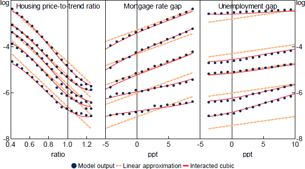
Note: Quantiles determined by varying the other variables.
3.1.2.1 Compromises
Ideally, the model used to calibrate the f (.) function would estimate total expected losses based on the expected size and duration of a given downturn. Unfortunately, the micro-simulation model we use is only able to estimate expected losses based on the expected size of the downturn (as it is a static model based on a cross-section of data). So we will likely overestimate the effect of short downturns and underestimate the impact of protracted downturns.
Moreover, MARTIN does not contain explicit equations for expectations. So we further compromise by assuming banks provision based on the contemporaneous extent of the deterioration; provisioning for losses will therefore be slower in our model than in reality.
With the micro-simulation model being much more detailed than our three-variable f (.) function, there are multiple determinants of expected losses that we (at best) implicitly capture via their relationships with our three included variables. For example, the influence of households' loan-to-valuation ratios (LVRs) and prepayment buffers at their 2017/18 surveyed levels is implicitly captured within the modelled relationships between the three included variables and expected losses (e.g. lower LVRs would mute the marginal effect of housing price declines on losses). However, this static and implicit capturing of average LVRs and prepayment buffers means any beneficial effect slower credit growth might have on improving resilience to future shocks will not be modelled (e.g. Schularick and Taylor 2012).
Endogenising households' resilience would be a fruitful avenue for future model development. In the meantime, to ensure households' resilience is at least exogenously updated, we recommend that Equation (2) be re-calibrated with each new SIH wave, and that users of this model be aware that any non-modelled changes that have occurred between the survey and the point of the shock will not be captured.
3.2 Total loan losses
We do not currently model losses on business loans, and simply assume business loan losses move proportionately with housing loan losses. This is obviously unrealistic. But we are not currently able to include a model for business loan losses as MARTIN does not currently have equations for business credit growth or commercial property prices, and the RBA is currently reviewing its business loan stress testing framework.
So that a model for business loan losses can be easily incorporated once the necessary components have been developed, we set business loan losses equal to some calibrated multiple of household loan losses:
And define total losses as:
where and have the business loan equivalent definitions of Equation (1), and is the household share of banks' outstanding loans (estimated from APRA data). Once an equation for business loan losses has been developed, the only change that needs to be made is to substitute this new equation for Equation (5).
In the meantime, is calibrated such that, in a downturn equivalent to what APRA assumed in their 2017 stress testing exercise, the sum of quarterly losses equals the total loan losses in APRA's exercise (APRA 2018).
3.3 Risk-weighted assets
For capital adequacy purposes, assets are risk weighted; if banks have riskier assets on their balance sheets, they need more capital to meet regulatory capital requirements. Risk weights are determined by a combination of APRA and the banks' perceptions of default probabilities and probable losses (APRA 2020). They therefore tend to co-move with losses but stay elevated longer than losses (RBA 2017).[7] To capture this extended cyclicality in a simple way, we model risk weights as an autoregression nonlinearly shocked by losses:
In reality, risk weights differ by asset class. Since we don't incorporate detailed asset mix data into BA-MARTIN, the risk-weight multiplier we use ( wt ) is the weighted-average value such that when multiplied by total assets at the beginning of the next period ( At+1 ) the resulting value equals the value of the banking system's risk-weighted assets.
With , an increase in losses causes an increase in wt; risk weights will continue to grow as long as losses are larger than the steady-state level . Once losses fall back to their steady-state level, the will cause the risk-weight multiplier to slowly move back to its steady state of (higher values of increase the speed of adjustment).
We calibrate based on banks' average risk weights during 2019. We calibrate and such that, when we input the losses from APRA's 2017 stress tests, Equation (7) produces a path of risk weights that approximately replicates the APRA stress test path.
3.4 Debt funding costs
Australian banks' high-interest deposit and non-deposit debt funding spreads have historically been determined more by liquidity/risk conditions in global funding markets than by domestic economic conditions (Brassil et al 2018). But increases in credit risk would increase banks' cost of debt funding. When the cash rate is sufficiently far above zero, we model these spreads as an exogenous random walk (to reflect the exogenous global markets and any other exogenous changes to these spreads) plus a term that increases with credit risk.
As in Major (2016), we model increases in credit risk as being linearly related to deteriorations in banks' capital adequacy. Using a panel regression of bond market spreads on capital ratios, Major found that a 1 percentage point fall in a bank's capital adequacy ratio is expected to increase its debt funding costs by 10 basis points; we calibrate our model to match this estimate.[8]
3.4.1 Zero lower bound
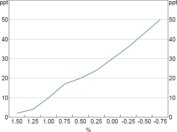
Retail deposit rates tend to have a lower bound around zero – due to the possibility of holding physical currency instead. Some bank deposits always pay near-zero interest. The lower bound does not matter much for these non-interest bearing accounts because banks hedge the fixed interest rate risk of these deposits using a ‘replicating portfolio’ hedge (Brassil et al 2018).
For deposit accounts that typically pay an above-zero rate of interest, this lower bound would bind only after the cash rate falls below a certain level. As it is costly to effectively hedge against an occasionally binding lower bound, banks remain exposed to this funding risk. The result is that banks' costs of funding fall by less than the cash rate once the cash rate moves below a certain level; in other words, the spread between the cash rate and banks' cost of funding increases as the cash rate falls.
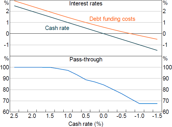
We use the information in Garner and Suthakar (2021) and discussions with RBA staff to model the increasing share of deposits at the lower bound as the cash rate falls below 1.5 per cent (Figure 3). How we incorporate this information into the BA-MARTIN equation for debt funding costs ( rD,t ) is explained in the Online Appendix. And the effect of the lower bound on monetary policy pass-through is explored in Section 5.[9]
3.5 Interest income
The lending spreads banks charge above their costs of debt funding have historically been unrelated to the level of interest rates (see Graph 13 in Garner and Suthakar (2021)). So we assume that when banks' capital ratios are at their desired level, they charge borrowers an exogenous spread above their costs of debt funding. We call these exogenous spreads ‘unconstrained lending spreads’, and model them as random walks – the unconstrained business spread is sB,t and the unconstrained housing spread is sM,t .[10]
When capital ratios fall below banks' desired levels, banks increase the spreads they charge borrowers above these unconstrained spreads. How banks respond to these capital deteriorations is explained in Section 3.8.
3.6 Profits (return on assets)
Banks' profits comprise their net non-interest income plus net interest income, less their loan losses (all after tax). For our purposes, it is sufficient to define banks' return on assets (ROA = profits / assets) rather than their profits.
Banks' net interest margins (net interest income as a share of assets) equal their average lending rates ( rA,t ), minus their average debt funding costs ( rD,t ) times their debt-to-assets ratio (equivalently defined as one minus their capital-to-assets ratio ( Et / At )). Using this definition and the previously defined losses variable ( Lt ), banks' return on assets ( ROAt ) is defined as:
where is one minus the corporate tax rate, represents banks' net non-interest income as a share of assets (assumed constant for simplicity), and banks' NIMs are divided by 400 because the model is quarterly and MARTIN interest rates are in annual percentage units.[11]
The NIM can be equivalently written as the net interest spread ( rA,t – rD,t ) plus the product of debt funding costs and the capital ratio. The net interest spread equals the weighted average of the unconstrained mortgage and business lending spreads plus any endogenous increase in spreads that results from banks wanting to improve their capital ratios following a deterioration (defined as ).[12] Substituting these definitions into the first line of Equation (8) is how we get to the second line.
3.7 Capital adequacy ratio
Using the asset risk-weight multiplier ( wt ), the capital-to-risk-weighted assets ratio at the beginning of period . The change in this ratio can be decomposed as (this decomposition is the discrete-time version of the total derivative):
We use the existing MARTIN equation for household credit growth (Equation (19) in the Online Appendix of Ballantyne et al (2019)) as a proxy for all credit growth (since MARTIN does not have a business credit growth equation). MARTIN's household credit growth equation can be written as a function of the contemporaneous mortgage rate and other endogenous and exogenous variables:
where Xt is a vector of the ‘other’ endogenous and exogenous variables in the household credit growth equation (these variables are all determined in period t or earlier, and include lags of the mortgage rate is the MARTIN-estimated contemporaneous effect of the mortgage rate on household credit growth, and B is a vector of coefficients defined in MARTIN.[13]
The change in capital / assets equals banks' return on assets ( ROAt ) plus new raisings of capital from external sources as a share of assets ( ENew,t / At ) minus the share of dividend payments ( Dt / At ).
Substituting all of the above into Equation (9) gives the following approximation:
Equation (11) is an approximation because we replace the et+1 interaction with credit growth (in Equation (9)), with et. This approximation ensures that the right-hand side of Equation (11) is a function of variables from period t or earlier ( is a function of lagged variables).[14]
3.7.1 State dependence
There are three as yet undefined endogenous variables in Equation (11): banks' new raisings of capital from external sources ( ENew,t ), their dividend payments ( Dt ), and within ROAt and is how banks increase their lending spreads in response to a capital deterioration . How banks set will be explained in Section 3.8. How banks set ENew,t and Dt depends on the state of the economy.
We assume that, when banks' capital adequacy ratios fall below target (i.e. when losses are sufficiently high), the cost of raising new capital would be sufficiently prohibitive that banks would not choose this option. We further assume that with capital adequacy below target, banks would retain as much of their earnings as possible – so banks would not pay dividends. Therefore, in what we call the ‘stressed state’, ENew,t = Dt = 0.
Outside of the stressed state, in what we call the ‘unconstrained state’, we assume banks are able to access external capital markets, and do so such that any demand-driven credit growth has no effect on their capital adequacy . In other words, external capital markets are accessed to fund new lending.[15]
Banks spend most of their time in the unconstrained state. And, as noted above, entry into the stressed state occurs when losses push banks' capital adequacy ratios below target. But it's not necessarily the case that the cost of raising new capital remains prohibitive for the entire time capital ratios remain below target (i.e. banks may re-enter the unconstrained state before their capital adequacy ratios return to their target levels). To capture this flexibility in our model, we allow the user to set the number of periods for which the stressed state lasts (see the Online Appendix for details).
We assume dividends remain at zero while capital adequacy is below target. Once capital returns to target, we assume dividends are set such that whenever Equation (11) would otherwise be positive. In other words, banks pay out excess profits as dividends.
It is worth noting that the lack of recent periods of extreme banking stress in Australia make it difficult to determine exactly how banks would respond in such a scenario. The assumptions we make around external capital raisings and dividend payments, which are consistent with the RBA's stress testing framework (RBA 2017), should therefore be seen more as prudent modelling choices that ensure we do not underestimate the financial accelerator effect, rather than exactly how banks would behave.
3.8 Credit supply
Consistent with the RBA's stress testing framework (RBA 2017), we assume banks only restrict credit supply in response to a capital shortfall. If we define banks' target for their capital adequacy ratio as , then if banks do not restrict credit supply their capital shortfall in period t +1 can be defined as:
where is defined as the value of (from Equation (11)) given the period ( t ), value of the credit supply response , and state of the economy (St).[16]
Now suppose banks restrict credit supply such that their capital shortfall in period t +1 is smaller than suggested by Equation (12):
where can be interpreted as the desired/required speed at which the capital adequacy ratio returns to target. If , Equation (13) simplifies to ; that is, there is no credit supply response and the speed at which the capital adequacy ratio returns to target is determined by P(t,0,St). If , credit supply is sufficiently restricted such that the capital ratio is returned to target within one period . If , credit supply is restricted such that the capital ratio is returned to target faster than P(t,0,St), but at a rate that allows a persistent capital shortfall.
By solving for the value of such that banks' capital ratios return to target at the speed defined in Equation (13) (i.e. setting the unique credit supply reduction that satisfies this equality is:[17]
In other words, the speed of adjustment uniquely determines how much banks increase their lending rates in response to a deterioration in capital adequacy. And these endogenously set lending rates combine with MARTIN's credit growth equation (Equation (10)) to determine the resulting rate of credit growth in the economy.
3.8.1 Calibrating the speed of adjustment
We calibrate so that banks return their capital ratios to target with a speed of adjustment that broadly matches the speed implied by the RBA's stress testing framework. In their framework, capital ratios return to target around 2–3 years from the downturn. So we approximate this by setting (Figure 4).
The amplification through the banking sector is clear in Figure 4. Following the initial shock, higher credit supply responsiveness leads to higher household and business lending rates and a faster return of capital to target. But the higher lending rates increase repayment burdens, reduce housing prices and investment, and increase unemployment, leading to higher losses. These losses further increase lending rates (relative to the counterfactual), and so on.[18]
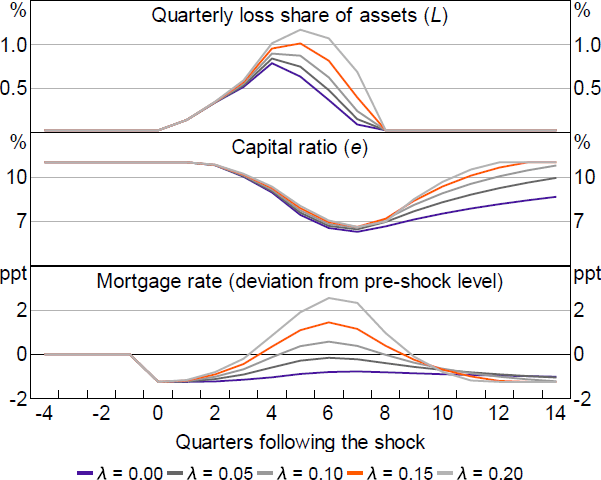
Notes: The shock is consistent with the shock used by APRA in their 2017 stress testing exercise (APRA 2018) – a 35 per cent fall in housing prices and unemployment increasing 5 percentage points. The cash rate is held constant following the initial policy response to the shock (125 basis points, as in the stress testing exercise).
3.8.2 Banks' choices have aggregate demand externalities
When determining how banks set their credit supply responses, it's important to differentiate between the variables each bank determines solely through their own choices, and the variables that depend on the choices made by all banks. This is because, even if all banks make the same choices in equilibrium, in a competitive system each bank treats the choices made by other banks as independent of their choice.[19] The result is that banks make different choices to what a monopolist would choose, thereby causing what is known as an ‘aggregate demand externality’.
In our model, these externalities amplify the financial accelerator mechanism. While each bank accounts for the effect their interest rate decision has on their NIM and credit growth, losses and risk weights are mostly determined by aggregate variables – such as housing prices and unemployment – and therefore depend on the decisions made by all banks.[20] Given that credit supply reductions amplify losses, these externalities lead to larger losses than if banks internalised the effects their combined decisions had on losses.
Figure 5 shows the effect of these externalities on the speed at which capital ratios return to target. The maroon bars show the effect of banks' credit supply decisions on NIMs and credit growth (i.e. the effects banks internalise), while the blue and orange bars show the effects these credit supply decisions have on losses and risk weights. During the peak of the stressed period, these extra losses and risk weights work against the NIM and credit growth changes, such that banks' capital ratios do not actually change much with the reduced credit supply. It is only when losses normalise that capital ratios increase at a noticeably faster speed.

To be absolutely clear, each bank's credit supply reduction still improves its capital ratio at the speed required by Equation (13). To explain why, suppose we looked at the Figure 5 equivalent for an individual bank. If this bank did not reduce its credit supply but all other banks did, then it is only the maroon bars that would be removed, the blue and orange bars would remain; the size of the maroon bar in period t equals the extra speed of adjustment required by Equation (13) .
3.8.3 Credit supply reduction affects new loans only
With this alternative assumption, banks' credit supply reductions have only marginal direct effects on their NIMs (as NIMs are determined by outstanding loans). Therefore, banks are only able to directly increase their capital ratio by reducing credit growth (i.e. through the denominator of the capital ratio). With the credit supply reduction working through the denominator only, achieving the same increase in the capital ratio requires a much larger reduction in credit supply, resulting in a much larger financial accelerator mechanism than with our baseline assumption.
Only minor changes to BA-MARTIN are required to implement this alternative assumption. This is because the original MARTIN relationship between household credit growth and lending rates remains unchanged (as it is determined by the lending rates available for new loans). With this credit growth-lending rates relationship unchanged, the endogenous credit supply reduction can still be implemented in BA-MARTIN via , but the interpretation of may become more nuanced (explained in more detail below). The changes required to BA-MARTIN are:
The direct effect of interest rates on losses occurs because increases in the interest rates of outstanding loans increase households' interest burdens and therefore increase the proportion of households unable to continue making payments. With only affecting new loans in this scenario, it is the mortgage rate gap without the credit supply reduction that enters the losses equation (Equation (15)).[21] NIMs are also determined by outstanding loans, so also needs to be removed from banks' return on assets (Equation (16) defines return on assets after this removal).
With each bank's credit supply reductions now working through credit growth only, the unique credit supply response that achieves the desired/required speed of adjustment is Equation (17); this response is always larger than Equation (14).
The interpretation of in this new-loans-only scenario is ‘the weighted average increase in lending rates paid by new borrowers, with constant weights’. The constant weights part of this interpretation is important if, for example, banks reduce lending volumes more for riskier loans (i.e. lending standards are tightened). In this case, even though each borrower would be paying more for their loan, the proportion of new borrowers would shift towards those with lower risk; so average lending rates with shifting weights need not increase. To achieve the correct credit supply reduction in BA-MARTIN, must reflect the average increased borrowing costs at the previous weights.
4. How Might COVID-19 Have Affected the Banking Sector and What Feedback Would This Have Had on the Real Economy?
The May 2020 Statement on Monetary Policy (SMP) (RBA 2020c) presented three possible scenarios for how the Australian economy might have evolved following the onset of the COVID-19 pandemic. While the downside scenario did not eventuate, it provides a useful example to illustrate the mechanisms of BA-MARTIN because the scenario gave rise to very large increases in the unemployment rate, decreases in activity and declines in housing prices.
In any macro model, variables can be split into exogenous variables (those determined outside the model) and endogenous variables (determined by the modelled dynamics). Any scenario must start from a series of changes to the exogenous variables; these changes are known as ‘shocks’. To assess the amplifying effect of the banking sector, we use the same set of shocks as was used to produce the downside scenario. We then compare how the endogenous variables evolve in BA-MARTIN with how they evolved in MARTIN.[22]
In addition to using the same shocks, we assume the same profile for economic policies. This is obviously unrealistic, as both monetary and fiscal policies would respond differently if the economic outcomes were different. But the purpose of this section is to showcase the potential amplifying effect of a stressed banking sector to a plausible crisis, not to assess the effectiveness of policy responses.[23]
4.1 The downside scenario
Relative to the baseline scenario, the downside scenario assumed that the outbreak persisted for longer than expected or flared up again, which would have seen mandated restrictions on domestic activity eased more gradually, international travel restrictions in place for longer periods of time, and prolonged precautionary behaviour by consumers and businesses. The resulting recovery in GDP was expected to be slower than the baseline scenario, with longer lasting effects on household and business balance sheets, as well as persistent damage to employment and supplier relationships. The level of GDP in the downside scenario troughed at 12 per cent below the February 2020 SMP forecasts, while the unemployment rate peaked above 10 per cent and remained elevated for a long time (RBA 2020c).
4.2 The downside scenario in BA-MARTIN
4.2.1 Banking sector variables
Figure 6 shows the effects that the downside scenario has on the key banking sector variables in BA-MARTIN (loan losses and capital). The figure shows these effects under our baseline assumption that banks reduce credit supply by increasing lending rates on all loans, and our alternative assumption that banks reduce credit supply by restricting new lending. Under both assumptions, the downside scenario decline in GDP, increase in unemployment and fall in housing prices results in a large increase in loan losses. The initial increase in losses is sufficiently large that banks' capital ratios decline by 1–2 percentage points.
As discussed in Section 2.1, increasing interest rates on outstanding loans has a large effect on banks' NIMs, and is therefore a powerful tool for recouping capital when external capital markets cannot be accessed at a cost-effective price. Moreover, by spreading the cost of capital replenishment across new and existing loans, the financial accelerator mechanism is dampened. In Figure 6, this manifests in banks achieving their desired/required speed of capital restoration with lower additional losses than when restricting new lending.
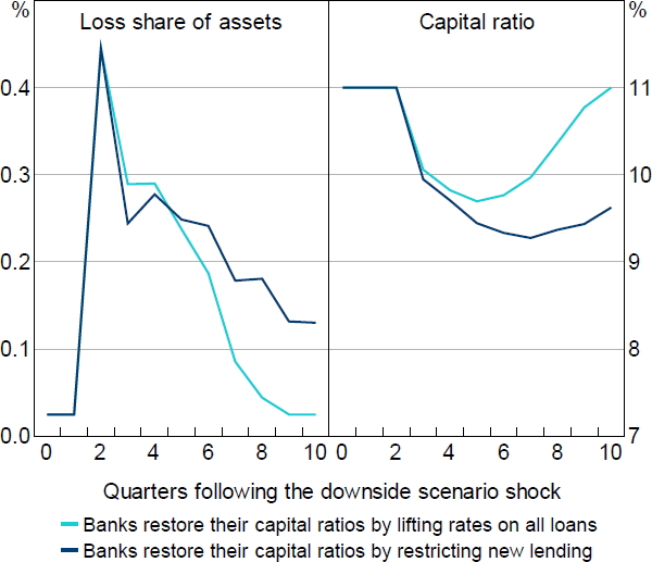
Because we calibrate to match the speed of aggregate capital ratio adjustment implied by the RBA's stress testing framework, the appropriate calibration if banks lift rates on all loans need not be the same as if banks restrict new loans only. We find that, when restricting new loans only, the larger credit supply restrictions required for each bank to achieve a given speed of adjustment lead to such magnified losses that the return of capital ratios to target takes longer (i.e. the aggregate demand externalities are larger). Therefore, approximating the RBA's stress testing framework requires a lower with the ‘restricting new loans only’ assumption. In this section, we set
Importantly, banks' capital ratios remain well above regulatory benchmarks under both credit supply assumptions (both the prudential minimum and regulatory capital buffer (RBA 2021)).
4.2.2 Credit supply response
The extent of the credit supply response to the downside scenario in BA-MARTIN can be measured by comparing the path for banks' lending rates and credit to what occurs when the same shocks are applied to MARTIN (Figure 7). When raising rates on all loans, achieving the capital ratio path shown in Figure 6 requires banks to increase their lending rates by 66 basis points. As banks' capital positions improve, banks begin to unwind this lending rate increase. In BA-MARTIN, this path of lending rates results in the level of credit provided to the economy being around 1.5 per cent lower than it would have been without the credit supply restriction.
Importantly, the estimated persistence of the economic variables in MARTIN (which is unchanged in BA-MARTIN) means that this lower level of credit persists well beyond the point that lending rates return to normal, which means that housing prices and economic activity would also be persistently lower. This is important for policymakers, as it means the economic cost of loan losses that are sufficiently high to engender a credit supply restriction lasts well beyond the point at which the credit supply restriction is removed.
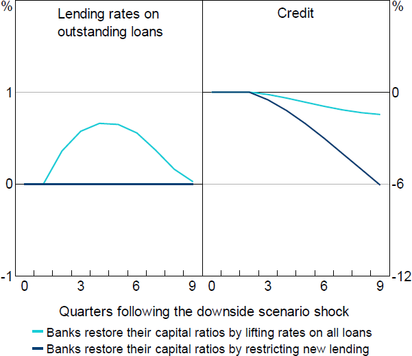
This persistent economic cost is much worse if banks decide to constrain new lending to restore their capital ratios.[24] Because a much larger credit supply restriction is required in this situation, credit is 6 per cent below the MARTIN level two years following the crisis. And if banks continue to find external capital raising difficult, this gap would continue to grow.
While examining deviations from MARTIN is the best way to analyse the financial accelerator mechanism, it is important to remember that these reductions in credit supply occur on top of already large reductions in credit demand (due to the original COVID-19 downside scenario shocks). We do not show their combined effect as the downside scenario profile for these variables were not made public with the May 2020 SMP.
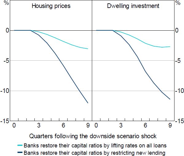
4.2.3 Effect on the housing market
Higher interest rates and lower credit growth dampen housing market activity. This dampening effect occurs both as a direct result of increasing the cost/reducing the availability of credit, and indirectly as the reduced housing market activity leads to lower income growth and higher unemployment (which feeds back into the banking sector and housing market).
When banks recapitalise by increasing lending rates on all loans, the path of interest rates causes housing prices to decline by an additional 3 per cent after two years (on top of the decline caused by the initial downside scenario shocks), which leads to a similar decline in dwelling investment (Figure 8). When banks restrict new lending, the larger reduction in credit supply results in housing prices and dwelling investment declining by around 12 per cent beyond the fall caused by the initial downside scenario shocks.
4.2.4 Effect on economic activity and unemployment
Figure 9 reproduces the scenarios from the May 2020 SMP and adds additional paths to show the amplification caused by the financial accelerator mechanism. When banks spread the credit supply response across all loans, the resulting increase in lending rates (which peaks at a 66 basis point increase) results in a small reduction in economic activity relative to the reduction caused by the COVID-19 shock itself. The level of GDP is around 0.3 per cent lower at the end of the forecast horizon, and unemployment is 0.1 percentage points higher (approximately 16,000 fewer employed people). While this amplification is small relative to the size of the COVID-19 shock, this increase in unemployment is highly persistent, lasting beyond the end of the forecast horizon.
Consistent with the much larger effects on the housing market, if banks restore their capital ratios by restricting new lending, the amplifying effect on economic activity is much larger. GDP would be around 1.3 per cent lower and the unemployment rate would be around 0.4 percentage points higher (approximately 59,000 fewer employed people).
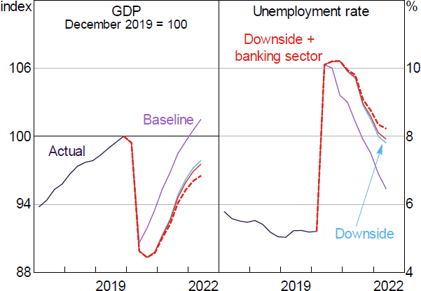
Note: Dashed line indicates when credit supply is restricted on new lending only.
Sources: ABS; Authors' calculations; RBA
It is worth reiterating that, in order to assess how much the banking sector can amplify the macroeconomic effects of crises, we explicitly prevent policy from responding to the amplification. In reality, monetary policy would respond by reducing the cash rate (or via unconventional policies), and it is likely that governments and APRA would also respond. How much monetary policy would need to respond may seem like a simple question – if lending spreads increase by 66 basis points, the effect on lending rates could be offset by reducing the cash rate by the same amount. But this does not account for the fact that the addition of a banking sector to MARTIN changes how monetary policy transmits through the economy, and introduces state-dependence. Assessing this state-dependent policy pass-through is the focus of the next section.
5. How Does the Pass-through of Monetary Policy Change with the State of the Economy?
In this section, we detail how the deposit rate lower bound dampens the pass-through of cash rate changes to other interest rates in the economy once the level of the cash rate moves below 1.5 per cent. We also explain how a deterioration in banks' capital adequacy may also change the pass-through of monetary policy. We then construct scenarios to show how the responses of banks' lending rates and macroeconomic variables can depend on the level of the cash rate and banks' capital positions (i.e. state-dependence). To provide context for the results, we compare the BA-MARTIN responses to those from the standard MARTIN model.
5.1 The mechanics of state-dependent pass-through
The pass-through of changes in the cash rate to lending rates in MARTIN has historically been one-for-one – that is, a 25 basis point decline in the cash rate reduces lending rates by 25 basis points – irrespective of the level of the cash rate. While this is a simplifying assumption incorporated within many macro models (see Appendix A), there is strong evidence that pass-through may deviate from one-for-one in low-rate and/or stressed environments.[25] The banking sector in BA-MARTIN facilitates a state-dependent transmission mechanism that more accurately reflects the true pass-through of policy rates to other interest rates in the economy.
There are several features of the banking system that can cause the pass-through of monetary policy to differ from one-for-one in some states (all of which are incorporated within BA-MARTIN).
5.1.1 Deposit rate lower bound
Most deposit accounts have an interest rate that typically moves with either the cash rate or longer term rates related to cash rate expectations. If banks are not willing to reduce retail deposit rates below zero because they fear a run to physical currency, then this typical co-movement with the cash rate will cease for these interest rates once they reach near zero. In other words, there may be a deposit rate lower bound that reduces the pass-through from cash rate changes to banks' funding costs, thereby reducing the pass-through to lending rates.
5.1.2 Banks' capital positions
As discussed in previous sections, in stressed states (i.e. when banks suffer large loan losses), banks may find it difficult to raise equity externally and may therefore rely on retained earnings and/or reduced lending to restore their capital ratios. A reduction in NIMs or increase in credit growth would slow this recapitalisation, while any reduction in losses would reduce the amount of recapitalisation that is required.
Cash rate reductions potentially lead to all three of these recapitalisation effects. So if banks desire/require a particular speed of recapitalisation, they may change lending spreads in response to the cash rate change, thereby changing pass-through. The NIM and credit growth effects reduce pass-through – banks would increase spreads in response to a cash rate reduction in order to increase NIMs and reduce credit growth – whereas the losses effect increases pass-through. Therefore, even the direction of the change in pass-through will depend on the state of the economy.[26]
In addition to this pass-through change that results from banks endogenously responding to the effect the cash rate change has on their capital ratios, banks' creditors might also respond to lower capital ratios by increasing the risk compensation they require when lending to banks. So any change in banks' capital ratios that results from a change in the cash rate (via the three recapitalisation effects) may also lead to an change in debt funding costs, thereby changing the pass-through of the cash rate to lending rates.[27]
5.2 Pass-through to banks' lending rates
The combination of all the above channels leads to a complex relationship between the state of the economy and interest rate pass-through – where even the direction of the pass-through (from the usual one-for-one) depends upon the state of the economy. To illustrate these relationships, we explore the state-dependence of pass-through using four scenarios:
- Illustrating the deposit lower bound mechanism with capital ratios remaining at target.
- Elevated losses cause a capital shortfall but deposit rates remain above their lower bound.
- Elevated losses cause a capital shortfall and some deposit rates reach their lower bound.
- Our alternative assumption in which banks respond to a capital shortfall by restricting the supply of new loans only (so pass-through differs between new and outstanding loans).
In Scenarios 2 to 4, the economy suffers an equivalently sized downturn (27 per cent fall in housing prices and unemployment rising 3 percentage points). This ensures that in each scenario the economy is in the same ‘state’ before monetary policy is changed. Importantly, changing the initial state will change the pass-through of monetary policy, so this section should be interpreted as illustrating how pass-through can change in a small number of possible scenarios. Moreover, all scenarios start from a benign economic position before the downturn occurs. If the economy is still recovering from a previous downturn, pass-through could deviate even further from the scenarios we explore.
5.2.1 Scenario 1: the deposit lower bound mechanism
Based on our estimates of the increasing share of deposits reaching their lower bound as the cash rate falls (Figure 3), Figure 10 shows how pass-through to debt funding costs is expected to fall as the cash rate falls below 1.5 per cent. Assuming banks' capital ratios remain at their desired level, changes to debt funding costs pass through one-for-one to household and business lending rates.[28] So as the cash rate declines below 1.5 per cent, this muted pass-through to debt funding costs leads to an equivalently muted pass-through to lending rates.
Note: Non-deposit debt funding costs are assumed to retain their one-for-one pass-through.
5.2.2 Scenario 2: capital shortfall when deposit rates remain above their lower bound
In stressed scenarios (i.e. when banks cannot raise capital externally), cash rate reductions inhibit recapitalisation by reducing NIMs and increasing credit growth (henceforth, the direct channel). However, these cash rate reductions also reduce unemployment and interest payments, and increase housing prices, thereby reducing bank losses and increasing banks' capital (henceforth, the indirect channel).
When the economy is in a benign economic position before the downturn occurs, we find that the indirect channel is the more powerful channel. Cash rate cuts therefore reduce banks' recapitalisation needs, allowing for competitive pressures to reduce lending spreads.[29] As a result, the pass-through of monetary policy exceeds 100 per cent (Figure 11).
For the direct channel to dominate, banks' capital shortfalls would need to be large relative to any newly provisioned losses. This would require a scenario in which banks previously provisioned heavily, causing a capital shortfall, but retained both the capital shortfall and the inability to raise equity externally even after provisioning returned to normal – in other words, the economy would not be starting from a benign economic position. The ‘excluding losses effect’ in Figure 11 illustrates the less than 100 per cent pass-through that would result in this situation.
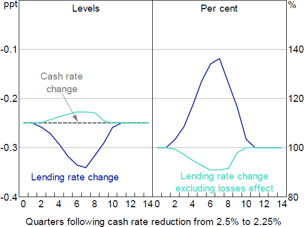
Figure 11 also shows how pass-through evolves over time. The point at which pass-through reaches its peak depends on the profile for losses (which depends on the shocks that hit the economy) and the point at which monetary policy changes. In our example, the cash rate is cut when the downturn hits the economy. Peak pass-through is not reached for another seven quarters; this is due to the delayed effect cash rate changes have on unemployment and housing prices in MARTIN.
Over time, as the economy begins to improve and losses return to normal, the beneficial effect of lower losses wanes and pass-through moves back towards 100 per cent. In our example, capital returns to target around the same time as losses normalise, such that pass-through does not move below 100 per cent. Situations in which capital shortfalls and an inability to obtain external equity persist longer than the point at which losses normalise would see pass-through temporarily move below 100 per cent before returning to normal.
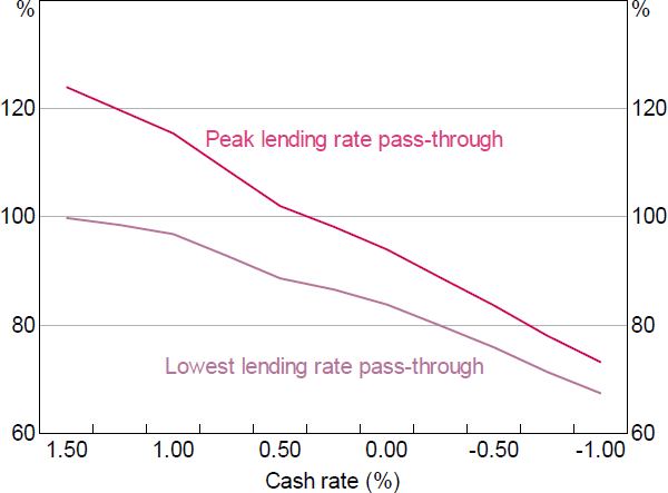
5.2.3 Scenario 3: capital shortfall with some deposit rates reaching their lower bound
The existence of a lower bound for deposit rates means interest rate pass-through falls as deposit rates progressively reach their lower bound (as shown in Scenario 1). When the cash rate gets very low, the deposit lower bound outweighs the indirect channel described in Scenario 2. So at very low rates, even the peak pass-through is far less than 100 per cent (Figure 12), while the lowest pass-through will closely follow the pass-through in Scenario 1.
In this scenario, we do not consider the effect of policies designed to directly influence longer-term interest rates (such as bond purchases, yield curve targeting or forward guidance). Moreover, any policies designed to directly reduce banks' non-deposit debt funding costs (e.g. the Term Funding Facility) would also have a large effect on lending rates, potentially offsetting the effect of the deposit rate lower bound. These policies can be accounted for in BA-MARTIN by exogenously lowering debt funding costs.
5.2.4 Scenario 4: banks restrict supply of new loans only
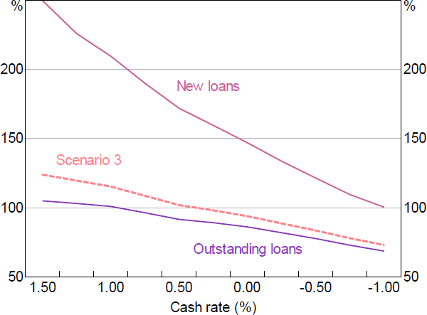
As discussed in previous sections, since restricting the supply of new loans does not immediately benefit banks' NIMs, achieving the same speed of capital ratio restoration as when all lending rates are increased requires a larger credit supply response. Therefore, the causal effect that cash rate changes have on banks' capital ratios (via the direct NIM and credit growth channel, and the indirect losses channel) will have a much larger effect on the pass-through to new loans than was the case when rates on all loans were adjusted (i.e. relative to Scenarios 2 and 3), while the pass-through to outstanding loans will be lower than was seen in Scenarios 2 and 3 (Figure 13).[30]
5.3 Pass-through to the economy
Since the addition of the banking sector to MARTIN changes how lending rates and credit growth respond to changes in the cash rate (in some states of the economy), it will also change how other macroeconomic variables respond to monetary policy. This section analyses the macroeconomic implications of the state-dependent pass-through scenarios from Section 5.2.
Figure 14 shows the responses of GDP, consumption and dwelling investment to an exogenous 25 basis point cash rate reduction that persists for the entire period of analysis; the responses we show are consistent with Scenarios 2 to 4 in Section 5.2. To show the effect of having a banking sector, these responses are shown for both BA-MARTIN and MARTIN.
The overall differences between the MARTIN and BA-MARTIN responses are a straightforward mapping from the discussion in Section 5.2. When deposit rates are away from their lower bound (left-hand panels), the responses in BA-MARTIN are larger than in MARTIN due to the beneficial indirect channel dominating the deleterious direct channel. This is amplified when banks restore their capital ratios by restricting the supply of new loans only.
However, while the overall differences are a straightforward mapping, the response profiles are not. This is because the profiles depend not only on how the pass-through to interest rates evolves over the cycle, but how persistent the effect of changes in interest rates are on different parts of the economy. This is why, even after accounting for the differences in scale, the response profile of dwelling investment is noticeably different to consumption and GDP.
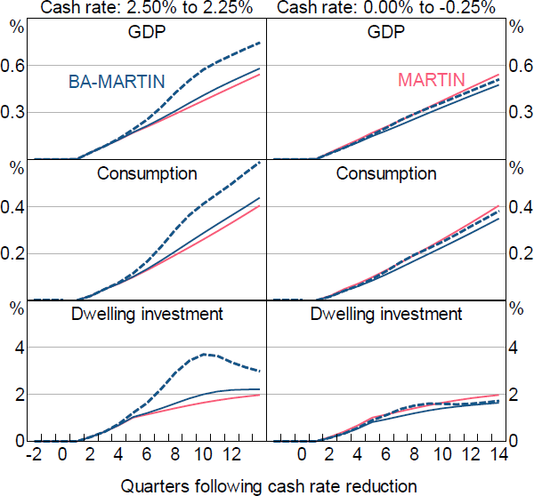
Notes: BA-MARTIN solid lines are the responses when banks reduce credit supply by changing interest rates on all loans, dashed lines are the responses when banks reduce the supply of new loans only. Banks are assumed to be unable to access external capital markets until losses normalise.
Once a sufficient proportion of deposit rates have reached their lower bound (right-hand panels), the reduced pass-through leads to smaller responses in BA-MARTIN than in MARTIN – consistent with Figure 12 showing that even the peak pass-through is less than 100 per cent when reducing the cash rate from 0 to –0.25 per cent. In the top right-hand panel, the response of GDP to the cash rate reduction is around 12 per cent smaller in BA-MARTIN than in MARTIN (when credit supply changes are implemented via all loans).
Figure 15 shows the responses of unemployment and inflation to the same exogenous changes in the cash rate as above. The high degree of estimated persistence embedded in these variables mutes the effect of the state-dependent pass-through. When the cash rate is above the point at which deposits increasingly reach their lower bound (left-hand panels), the inflation and unemployment responses are 7–9 per cent larger than in MARTIN (when credit supply changes are implemented via all loans). The effect of the deposit lower bound has a more noticeable effect on pass-through (right-hand panels); the inflation and unemployment responses are 10–12 per cent smaller than in MARTIN.
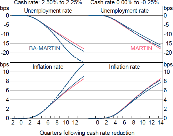
Notes: BA-MARTIN solid lines are the responses when banks reduce credit supply by changing interest rates on all loans, dashed lines are the responses when banks reduce the supply of new loans only. Banks are assumed to be unable to access external capital markets until losses normalise.
Our analysis in this section produces two broad implications for monetary policy. First, the persistence of macroeconomic variables mutes the effects the temporary lending rate pass-through amplifications have on economic activity, the labour market and consumer prices. Second, the deposit lower bound causes an economically significant and persistent reduction in expansionary policy pass-through when the level of interest rates is sufficiently low. The welfare implications of this reduced pass-through are not simply the differences between the MARTIN and BA-MARTIN curves at each point in time, but the cumulative difference. So it is important for policymakers to take this reduced pass-through into account when formulating policy.
In this section we have only considered the effectiveness of policy designed to expand economic activity. But an important implication of the deposit lower bound is that it has the opposite effect on the pass-through of policy tightening. As the cash rate is increased from these low levels, the interest paid on deposit accounts is expected to move away from the lower bound, causing a stronger tightening than if these deposit rates had remained at the lower bound.
6. Conclusion
We have built an extension to MARTIN that incorporates one of the key financial accelerator mechanisms – a banking sector that endogenously and nonlinearly changes credit supply in response to loan losses and/or changes to their funding costs. By combining a large and complex macroeconometric model with a micro-simulation model, and nonlinear stress testing and funding costs frameworks, our approach moves beyond the existing macroeconometric frontier.
We have shown that the ability to increase lending rates across new and outstanding loans – as is the case in Australia – provides a powerful capital restoration mechanism that means credit supply does not need to be reduced as considerably as if banks were confined to restricting new loans only. This finding highlights the importance of having a model that is designed specifically to capture the features of the Australian banking system (instead of relying on the experiences of stressed foreign banking systems), and has important implications for assessing the potential macroeconomic costs of banking system stress in Australia.
To ensure the features of the Australian system are captured as best as possible, an important avenue for future research is the explicit incorporation of business loan losses into BA-MARTIN (Section 3.2 explains why this is not yet possible). In recent history, business loans have been a larger driver of banks' losses than household loans (Rodgers 2015). By calibrating our model to APRA's stress testing results, we are able to capture business loan losses only to the extent that they are correlated with household loan losses. Our current approach is therefore far from ideal.
Two questions we have begun exploring in this paper are: ‘How can the banking sector amplify macroeconomic shocks in Australia?’ and ‘How can the banking sector change the pass-through of monetary policy?’ But the results presented here are only the beginning. The COVID-19 downside scenario from the May 2020 Statement on Monetary Policy is just one scenario out a wide range of plausible sources of stress. To properly evaluate how the banking sector can amplify macroeconomic shocks, a much wider range of possible shocks should be assessed.
Our analysis of how the banking sector can change the pass-through of monetary policy is similarly narrow. We assume the economy starts from a benign economic situation before it is ‘shocked’ in a way that stresses the banking sector and requires monetary policy to respond. The results are promising; monetary policy is more effective precisely when it needs to be. But this may not always be the case.
The amplified pass-through occurs solely due to the ability of policy to reduce losses. If the banking system begins in a stressed state, the fact that lower interest rates slow the capital restoration process (by decreasing NIMs and increasing credit demand) may dominate the beneficial effect of reducing further losses. In extreme cases, it may be that a lower cash rate slows capital restoration by so much that banks' endogenous credit supply responses more than offset the macroeconomic effect of the cash rate cut. The point at which this occurs is known as the ‘reversal rate’ (Brunnermeier and Koby 2018). Investigating the conditions that may give rise to a reversal rate in Australia is an important avenue for future research.
Having a banking sector within a macroeconomic model permits assessment of the potential complementarities or trade-offs between the RBA's inflation and full employment objectives and its financial stability objective. BA-MARTIN also provides an additional tool to help calibrate macroprudential policies. For example, a countercyclical capital buffer could be modelled as a temporary decline in banks' capital target , which would reduce the capital shortfall that banks try to make-up during the period of peak stress. Alternatively, APRA could give banks relief with respect to how quickly they expect capital to be restored following a crisis (i.e. reducing the speed of adjustment parameter .[31] In fact, by helping banks coordinate on a lower when losses are at their highest, APRA would be fulfilling the classic regulatory role of reducing negative externalities (see Section 3.8.2).
We look forward to seeing how BA-MARTIN is used in the future, but hope that its accuracy is never tested in reality.
Appendix A: Literature Review
The motivation for this project is clear. We know that feedback between the banking sector and real economy can be an important source of shock amplification, so we want a modelling framework that incorporates at least some of these financial accelerator channels. Unfortunately, the best way to incorporate these channels is not obvious.
While the existence of financial accelerator mechanisms was known before the global financial crisis (Kiyotaki and Moore 1997; Bernanke et al 1999), it was this crisis that highlighted the failure of modern macroeconomics to fully appreciate their size and likelihood of occurring (Lindé et al 2016; Gertler and Gilchrist 2018). While progress has been made, the macro literature has advanced in a myriad of different directions; from adding linear mechanisms (Gertler and Kiyotaki 2010; Christiano, Motto and Rostagno 2014), to applying numerical solution methods to small macrofinancial models with simple nonlinearities (He and Krishnamurthy 2013; Brunnermeier and Sannikov 2014; Adrian and Duarte 2016), and using atheoretical statistical techniques to find highly nonlinear relationships between macro and financial variables (Adrian, Boyarchenko and Giannone 2019a, 2019b; Hartigan and Wright 2021). Moreover, very few of these strands of literature take financial intermediation seriously; common approaches either explicitly ignore banks, do not model them realistically, or implicitly assume their influence is captured in the reduced-form parameters of the model (see Jakab and Kumhof (2018) for a discussion). Unfortunately, a unified theory of macroeconomics and finance still eludes us.
This gap between theory and reality also exists within the central bank modelling universe. Macroeconometric models at central banks either do not include a financial sector, or include only linear financial accelerator mechanisms (Adrian 2020; Muellbauer 2020). At the same time, areas in charge of financial stability have constructed complex nonlinear stress testing frameworks (Burrows, Learmonth and McKeown 2012; Adrian, Morsink and Schumacher 2020; Correia et al 2020). When discussing the relationship between the Bank of England's macro modelling framework and their financial stability modelling, Hendry and Muellbauer (2018, p 311) state that:
It seems as though the linkage is almost entirely one way, from the ‘real economy’ to finance. The contradictory lesson from the global financial crisis apparently remains to be learned …
The most well-known of these central bank macroeconometric models, FRB/US, developed by the Federal Reserve Board (Brayton, Laubach and Reifschneider 2014) abstracts from both financial accelerator mechanisms and the financial sector. This abstraction is also a feature of the key semi-structural policy models of the Bank of Canada, LENS (Gervais and Gosselin 2014); European Central Bank, ECB-BASE (Angelini et al 2019); the Bank of Japan, Q-JEM (Hirakata et al 2019); and the Reserve Bank of New Zealand, NZSIM (Austin and Reid 2017).
The semi-structural model developed by the Norges Bank, the Small Macro Model (SMM) (Hammersland and Træe 2014), incorporates a linear financial accelerator mechanism in which lower asset prices reduce collateral values, thereby restricting investment and amplifying the asset price fall (akin to the Kiyotaki and Moore (1997) and Bernanke et al (1999) mechanisms). The Central Bank of Chile's model, MSEP (Arroyo Marioli, Becerra and Solorza 2021), incorporates a linear financial accelerator in which credit growth and risk directly affect GDP growth, while GDP growth directly affects credit growth and risk. Importantly, neither of these models explicitly incorporate a banking sector nor stress in the financial system.
De Nederlandsche Bank's semi-structural model, DELFI 2.0 (Berben, Kearney and Vermeulen 2018), includes a comprehensive banking sector that has many similarities with our framework. However, they differ from our approach by modelling the banking sector using a linear error correction framework (including for loan losses and capital shortfalls), and by estimating the relationships rather than calibrating from existing models. The Bank of Italy's Quarterly Model, BIQM (Miani et al 2012), includes a banking sector that, like our framework, feeds back into the real economy via lending rates. But like DELFI 2.0, BIQM uses a linear framework with estimated relationships.
Some central bank stress testing frameworks include an amplifying feedback to the real economy. The Bank of Japan uses an estimated medium-scale model with a macroeconomic sector, and a financial sector split into individual institutions; they show that the inclusion of feedback mechanisms more than doubles the effect of a shock to GDP (Kitamura et al 2014). The European Central Bank uses several models to incorporate amplifying mechanisms within their stress testing framework (Henry and Kok 2013). While the financial sector amplification mechanisms these frameworks incorporate are similar to our proposal, their focus on stress testing means they have a more detailed financial sector than our proposal but a less detailed macroeconomic framework. Therefore, as far as we can tell, what we are attempting has not been done before.
References
Adrian T (2020), ‘“Low for Long” and Risk-Taking’, IMF Departmental Paper No 20/15.
Adrian T, N Boyarchenko and D Giannone (2019a), ‘Multimodality in Macro-Financial Dynamics’, Federal Reserve Bank of New York Staff Report No 903.
Adrian T, N Boyarchenko and D Giannone (2019b), ‘Vulnerable Growth’, The American Economic Review, 109(4), pp 1263-1289.
Adrian T and F Duarte (2016), ‘Financial Vulnerability and Monetary Policy’, Federal Reserve Bank of New York Staff Report No 804, rev September 2017.
Adrian T, J Morsink and L Schumacher (2020), ‘Stress Testing at the IMF’, IMF Departmental Paper No 20/04.
Altavilla C, L Burlon, M Giannetti and S Holton (2019), ‘Is There a Zero Lower Bound? The Effects of Negative Policy Rates on Banks and Firms’, European Central Bank Working Paper Series No 2289, rev June 2020.
Angelini E, N Bokan, K Christoffel, M Ciccarelli and S Zimic (2019), ‘Introducing ECB-BASE: The Blueprint of the New ECB Semi-structural Model for the Euro Area’, European Central Bank Working Paper Series No 2315.
APRA (Australian Prudential Regulation Authority) (2017), ‘APRA Announces “Unquestionably Strong” Capital Benchmarks’, Media Release, 19 July.
APRA (2018), ‘Testing Resilience: The 2017 Banking Industry Stress Test’, APRA Insight, 3.
APRA (2019), ‘Review of APRA's Prudential Measures for Residential Mortgage Lending Risks’, Information Paper, 29 January.
APRA (2020), ‘APRA Explains: Risk-weighted Assets’, APRA Insight, 2.
Arroyo Marioli F, JS Becerra and M Solorza (2021), ‘The Credit Channel Through the Lens of a Semi-Structural Model’, Documentos de Trabajo del Banco Central de Chile No 911.
Austin N and G Reid (2017), ‘NZSIM: A Model of the New Zealand Economy for Forecasting and Policy Analysis’, Reserve Bank of New Zealand Bulletin, 80(1).
Ballantyne A, T Cusbert, R Evans, R Guttmann, J Hambur, A Hamilton, E Kendall, R McCririck, G Nodari and D Rees (2019), ‘MARTIN Has Its Place: A Macroeconometric Model of the Australian Economy’, RBA Research Discussion Paper No 2019-07.
Bassett WF, MB Chosak, JC Driscoll and E Zakrajšek (2014), ‘Changes in Bank Lending Standards and the Macroeconomy’, Journal of Monetary Economics, 62, pp 23-40.
Berben R-P, I Kearney and R Vermeulen (2018), ‘DELFI 2.0, DNB's Macroeconomic Policy Model of the Netherlands’, De Nederlandsche Bank Occasional Studies, 16-5.
Bergmann M (2020), ‘The Determinants of Mortgage Defaults in Australia – Evidence for the Double-Trigger Hypothesis’, RBA Research Discussion Paper No 2020-03.
Bernanke BS (2018), ‘The Real Effects of Disrupted Credit: Evidence from the Global Financial Crisis’, Brookings Papers on Economic Activity, Fall, pp 251–322.
Bernanke BS, M Gertler and S Gilchrist (1999), ‘The Financial Accelerator in a Quantitative Business Cycle Framework’, in JB Taylor and M Woodford (eds), Handbook of Macroeconomics: Volume 1C, Handbooks in Economics 15, Elsevier, Amsterdam, pp 1341–1393.
Bilston T, R Johnson and M Read (2015), ‘Stress Testing the Australian Household Sector Using the HILDA Survey’, RBA Research Discussion Paper No 2015-01.
Brassil A, J Cheshire and J Muscatello (2018), ‘The Transmission of Monetary Policy through Banks' Balance Sheets’, in J Simon and M Sutton (eds), Central Bank Frameworks: Evolution or Revolution?, Proceedings of a Conference, Reserve Bank of Australia, Sydney, pp 73–122.
Brayton F, T Laubach and D Reifschneider (2014), ‘The FRB/US Model: A Tool for Macroeconomic Policy Analysis’, Board of Governors of the Federal Reserve System, FEDS Notes, 3 April.
Brunnermeier MK and Y Koby (2018), ‘The Reversal Interest Rate’, NBER Working Paper No 25406.
Brunnermeier MK and Y Sannikov (2014), ‘A Macroeconomic Model with a Financial Sector’, The American Economic Review, 104(2), pp 379–421.
Burrows O, D Learmonth and J McKeown (2012), ‘RAMSI: A Top-Down Stress-Testing Model’, Bank of England Financial Stability Paper No 17.
CGFS (Committee on the Global Financial System) (2019), Unconventional Monetary Policy Tools: A Cross-Country Analysis, CGFS Papers No 63, Bank for International Settlements, Basel.
Christiano LJ, R Motto and M Rostagno (2014), ‘Risk Shocks’, The American Economic Review, 104(1), pp 27–65.
Correia S, KF Kiernan, MP Seay and CM Vojtech (2020), ‘Primer on the Forward-Looking Analysis of Risk Events (FLARE) Model: A Top-Down Stress Test Model’, Board of Governors of the Federal Reserve System Finance and Economics Discussion Series No 2020-15.
Davies M, C Naughtin and A Wong (2009), ‘The Impact of the Capital Market Turbulence on Banks' Funding Costs’, RBA Bulletin, June, pp 1–13.
FSRC (Financial Services Royal Commission) (2018), Some Features of the Australian Banking Industry, Background Paper 1, (Hon Kenneth Hayne AC QC, Commissioner), Royal Commission into Misconduct in the Banking, Superannuation and Financial Services Industry, Canberra, 9 February.
Garner M and A Suthakar (2021), ‘Developments in Banks' Funding Costs and Lending Rates’, RBA Bulletin, March.
Gertler M and S Gilchrist (2018), ‘What Happened: Financial Factors in the Great Recession’, Journal of Economic Perspectives, 32(3), pp 3–30.
Gertler M and N Kiyotaki (2010), ‘Financial Intermediation and Credit Policy in Business Cycle Analysis’, in BM Friedman and M Woodford (eds), Handbook of Monetary Economics: Volume 3A, Handbooks in Economics, Elsevier, Amsterdam, pp 547–599.
Gervais O and M-A Gosselin (2014), ‘Analyzing and Forecasting the Canadian Economy through the LENS Model’, Bank of Canada Technical Report No 102.
Guerrieri V and H Uhlig (2016), ‘Housing and Credit Markets: Booms and Busts’, in JB Taylor and H Uhlig (eds), Handbook of Macroeconomics: Volume 2B, Handbooks in Economics, Elsevier, Amsterdam, pp 1427–1496.
Hack M and S Nicholls (2021), ‘Low Interest Rates and Bank Profitability – The International Experience So Far’, RBA Bulletin, June.
Hammersland R and CB Træe (2014), ‘The Financial Accelerator and the Real Economy: A Small Macroeconometric Model for Norway with Financial Frictions’, Economic Modelling, 36, pp 517–537.
Hartigan L and M Wright (2021), ‘Financial Conditions and Downside Risk to Economic Activity in Australia’, RBA Research Discussion Paper No 2021-03.
He Z and A Krishnamurthy (2013), ‘Intermediary Asset Pricing’, The American Economic Review, 103(2), pp 732–770.
Hendry DF and J Muellbauer (2018), ‘The Future of Macroeconomics: Macro Theory and Models at the Bank of England’, Oxford Review of Economic Policy, 34(1-2), pp 287–328.
Henry J and C Kok (eds) (2013), ‘A Macro Stress Testing Framework for Assessing Systemic Risks in the Banking Sector’, European Central Bank Occasional Paper Series No 152.
Hirakata N, K Kan, A Kanafuji, Y Kido, Y Kishaba, T Murakoshi and T Shinohara (2019), ‘The Quarterly Japanese Economic Model (Q-JEM): 2019 Version’, Bank of Japan Working Paper Series No 19-E-7.
Jakab Z and M Kumhof (2018), ‘Banks are Not Intermediaries of Loanable Funds – Facts, Theory and Evidence’, Bank of England Staff Working Paper No 761, rev June 2019.
Kearns J, M Major and D Norman (2020), ‘How Risky is Australian Household Debt?’, RBA Research Discussion Paper No 2020-05.
Kitamura T, S Kojima, K Nakamura, K Takahashi and I Takei (2014), ‘Macro Stress Testing at the Bank of Japan’, Bank of Japan Research Paper, October.
Kiyotaki N and J Moore (1997), ‘Credit Cycles’, Journal of Political Economy, 105(2), pp 211–248.
Lea M (2010), ‘International Comparison of Mortgage Product Offerings’, Research Institute for Housing America Research Report, 27 September. Available at <https://www.mba.org/assets/Documents/Research/RIHA/74023_10122_Research_RIHA_Lea_Report.pdf>.
Lindé J, F Smets and R Wouters (2016), ‘Challenges for Central Banks' Macro Models’, in JB Taylor and H Uhlig (eds), Handbook of Macroeconomics: Volume 2B, Handbooks in Economics, Elsevier, Amsterdam, pp 2185–2262.
Maddalonia A and J-L Peydró (2013), ‘Monetary Policy, Macroprudential Policy, and Banking Stability: Evidence from the Euro Area’, International Journal of Central Banking, 9(1), pp 121–169.
Major M (2016), ‘Estimating the Effect of Capital Ratios on Funding Spreads’, Unpublished manuscript, Reserve Bank of Australia, 27 October.
Miani C, G Nicoletti, A Notarpietro and M Pisani (2012), ‘Banks' Balance Sheets and the Macroeconomy in the Bank of Italy Quarterly Model’, Banca D'Italia, Questioni di Economia e Finanza (Occasional Papers) No 135.
Muellbauer J (2020), ‘Implications of Household-Level Evidence for Policy Models: The Case of Macro-Financial Linkages’, Oxford Review of Economic Policy, 36(3), pp 510–555.
RBA (Reserve Bank of Australia) (2012), ‘Graph 2.21: Credit Ratings of the Largest 100 Banking Groups’, Financial Stability Review, March.
RBA (2017), ‘Box D: Stress Testing at the Reserve Bank’, Financial Stability Review, October, pp 46–49.
RBA (2020a), ‘The Australian Financial System’, Financial Stability Review, October, pp 35–45.
RBA (2020b), ‘Box C: The Use of Banks' Capital Buffers’, Financial Stability Review, October.
RBA (2020c), ‘Economic Outlook’, Statement on Monetary Policy, May.
RBA (2021), ‘The Australian Financial System’, Financial Stability Review, April.
Rodgers D (2015), ‘Credit Losses at Australian Banks: 1980–2013’, RBA Research Discussion Paper No 2015-06.
Schularick M and AM Taylor (2012), ‘Credit Booms Gone Bust: Monetary Policy, Leverage Cycles, and Financial Crises, 1870–2008’, The American Economic Review, 102(2), pp 1029–1061.
Sparks K and M Garner (2021), ‘Bank Fees in Australia During the COVID-19 Pandemic’, RBA Bulletin, June.
Acknowledgements
For generously giving up their time to help us understand the bank modelling frameworks used by the RBA, we would like to thank Megan Garner, Nick Garvin, Lea Jurkovic, Marcus Miller, David Norman, Anirudh Suthakar, Dmitry Titkov and Callan Windsor. We would also like to thank Natasha Cassidy, Luci Ellis, Rochelle Guttmann, John Muellbauer, David Norman, Daniel Rees, Ivan Roberts, John Simon and participants at APRA, RBA and RBNZ seminars for their helpful comments and suggestions. The views expressed in this paper are those of the authors and do not necessarily reflect the views of the Reserve Bank of Australia. The authors are solely responsible for any errors.
Footnotes
We define ‘losses’ as the flow of provisions and unexpected loan write-offs (see Section 3.1 for further explanation). [1]
More accurately, we assume that when the whole banking system suffers a capital deterioration, the cost of raising new capital would be sufficiently prohibitive that banks would not choose this option. [2]
For simplicity, we assume there are barriers to entry, and that banks are homogeneous and suffer proportional capital deteriorations. With the majority of loans in Australia being variable-rate loans, we further simplify the model by assuming all loans have variable rates and that switching lenders is costless. Combined, these assumptions mean profit-maximising banks will maintain equivalent interest rates on new and outstanding loans in equilibrium (in reality, market power and switching costs permit a small differential between new and outstanding lending rates). [3]
We are implicitly assuming that over MARTIN's estimation period the credit supply curve was flat (i.e. the curve shifted with funding costs, but the interest rates set by banks were unrelated to quantities). This is a reasonable assumption for most of the estimation period, given Australian banks' persistently high credit quality. However, this assumption was likely violated during 2015–18, when quantity-based regulatory restrictions were placed on investor and interest-only loans (APRA 2019). [4]
Lags are used to avoid introducing circular references that would require us to adapt multiple existing MARTIN equations. Intuitively, the gap variables are designed to capture the fact that losses depend on how these variables evolve relative to long-run expectations. [5]
Distance to default is defined as a household's post-tax income (including transfers) after rent and loan payments, minus the Household Expenditure Measure (developed by the Melbourne Institute, and used as a minimum consumption benchmark). A household is assumed to be unable to service its mortgage once successive periods of negative ‘distance’ more than offset the household's liquid assets (e.g. balances in offset/redraw accounts). [6]
During COVID-19, for example, the major banks estimated that in some scenarios these procyclical increases in risk weights could have subtracted 70 to 180 basis points from their capital ratios (RBA 2020b). [7]
The Major (2016) estimates are derived from a linear model over a period during which the credit quality of the Australian banking sector remained high; so we likely underestimate the change in debt funding costs that would occur during an extreme stress scenario. [8]
In some jurisdictions, banks have increased fees to offset the deposit lower bound (Hack and Nicholls 2021). There is no evidence of this occurring in Australia at this stage (Sparks and Garner 2021). [9]
MARTIN does not incorporate interest rates for non-housing personal loans. Instead, the housing spread is used as a proxy for the spread on all household loans (more than 90 per cent of household loans are for housing). [10]
Although banks' net non-interest income is not constant, between 2004 and 2017 it had a constant mean (relative to assets) and exhibited little persistence (see Figure 11 in Brassil et al (2018)). [11]
We assume the credit supply response is imposed equally on household and business loans. [12]
will not simply equal the coefficient of the nominal mortgage rate in the household credit growth equation. This is because the real mortgage rate also appears in the credit growth equation; is time-varying because the difference between the nominal and real mortgage rates depends on the rate of inflation. [13]
This approximation means the approximate value of will equal the true value times . Therefore, as long as quarterly credit growth is close to zero, this approximation will not deviate too far from the true value. [14]
We assume banks only offset the demand-driven credit growth, which is defined as credit growth excluding any credit supply responses , since reducing external capital raisings to offset credit supply reductions would be counterproductive. [15]
zt has a subscript t because all determinants of the period t +1 capital shortfall are known in period t. [16]
Given that we are using MARTIN's household credit growth equation as a proxy for total credit growth, for the purposes of determining we assume the relevant interest rate for credit growth is rA,t (i.e. in Equation (10) we replace rM,t with rA,t for the purposes of determining ). [17]
Even with , the mortgage spread to the cash rate increases in Figure 4 (i.e. the purple line rises despite a constant cash rate). This is due to the effect of the capital deterioration on debt funding costs. [18]
With four major banks, each of the majors would likely account for the effects of their decisions on aggregate variables. So treating the Australian system as perfectly competitive is a simplification. [19]
Solving for the value of that satisfies Equation (13) is approximate to solving for each bank's infinite-horizon optimal credit supply (for a given ). This is because the effects that banks internalise (NIMs and credit growth) are close to independent of past values of z* (the small dependency is shown in the ‘Other’ bar in Figure 5), while the effects they do not internalise (losses and risk weights) and that appear in Equation (13) are independent of . [20]
Importantly, losses will still increase indirectly via the lower housing prices and higher unemployment caused by the credit supply reduction. [21]
To be clear, banking sector stress was incorporated into the downside scenario using the judgement of RBA staff. Our use of this scenario is to illustrate the new BA-MARTIN mechanisms, not to change the scenario itself. [22]
MARTIN incorporates an endogenous policy response. So our policy assumption in this section should be seen as an explicit aberration for ease of exposition, rather than the way BA-MARTIN typically works. [23]
We do not show the observed increase in lending rates when restricting new loans only because the size of the increase would depend on how the restriction is implemented (e.g. if lending volumes are reduced more for riskier loans, see Section 3.8.3). The reduction in credit is shown as it will not differ between implementations. [24]
See CGFS (2019), Altavilla et al (2020) and Hack and Nicholls (2021) for international evidence. Our focus is on the cash rate pass-through excluding unconventional policies that work through other interest rates. [25]
It is theoretically possible for the NIM and credit growth effects to be so strong that lending spreads increase by more than the cash rate reduction. The point at which this occurs is known as the ‘reversal rate’ (Brunnermeier and Koby 2018). We leave investigation of the reversal rate in Australia for future research (see Section 6). [26]
The cost of deposits is also affected as banks compete for deposit funding when faced with more expensive wholesale funding. [27]
MARTIN assumes all loans are variable-rate loans, so this pass-through immediately affects all outstanding loans. [28]
This does not imply that banks could improve their capital positions by reducing lending spreads. For a given reduction in lending rates, the difference between this reduction occurring via the cash rate and via lending spreads is that a cash rate reduction has a much smaller effect on NIMs than a reduction in lending spreads. [29]
How to quantify pass-through when credit supply is restricted differently across borrowers (e.g. a tightening of lending standards) is not obvious. We measure pass-through via the implied effect on explained in Section 3.8.3. The pass-through to outstanding loans may still differ from 100 per cent due to the deposit lower bound and banks' creditors changing their required risk compensation. [30]
A pre-emptive example of such a policy was APRA's announcement that, following COVID-19, ‘its future expectations for capital will allow banks to rebuild their capital buffers in an orderly manner’ (RBA 2020a). [31]