RDP 2022-01: MARTIN Gets a Bank Account: Adding a Banking Sector to the RBA's Macroeconometric Model 4. How Might COVID-19 Have Affected the Banking Sector and What Feedback Would This Have Had on the Real Economy?
January 2022
- Download the Paper 1,775KB
The May 2020 Statement on Monetary Policy (SMP) (RBA 2020c) presented three possible scenarios for how the Australian economy might have evolved following the onset of the COVID-19 pandemic. While the downside scenario did not eventuate, it provides a useful example to illustrate the mechanisms of BA-MARTIN because the scenario gave rise to very large increases in the unemployment rate, decreases in activity and declines in housing prices.
In any macro model, variables can be split into exogenous variables (those determined outside the model) and endogenous variables (determined by the modelled dynamics). Any scenario must start from a series of changes to the exogenous variables; these changes are known as ‘shocks’. To assess the amplifying effect of the banking sector, we use the same set of shocks as was used to produce the downside scenario. We then compare how the endogenous variables evolve in BA-MARTIN with how they evolved in MARTIN.[22]
In addition to using the same shocks, we assume the same profile for economic policies. This is obviously unrealistic, as both monetary and fiscal policies would respond differently if the economic outcomes were different. But the purpose of this section is to showcase the potential amplifying effect of a stressed banking sector to a plausible crisis, not to assess the effectiveness of policy responses.[23]
4.1 The downside scenario
Relative to the baseline scenario, the downside scenario assumed that the outbreak persisted for longer than expected or flared up again, which would have seen mandated restrictions on domestic activity eased more gradually, international travel restrictions in place for longer periods of time, and prolonged precautionary behaviour by consumers and businesses. The resulting recovery in GDP was expected to be slower than the baseline scenario, with longer lasting effects on household and business balance sheets, as well as persistent damage to employment and supplier relationships. The level of GDP in the downside scenario troughed at 12 per cent below the February 2020 SMP forecasts, while the unemployment rate peaked above 10 per cent and remained elevated for a long time (RBA 2020c).
4.2 The downside scenario in BA-MARTIN
4.2.1 Banking sector variables
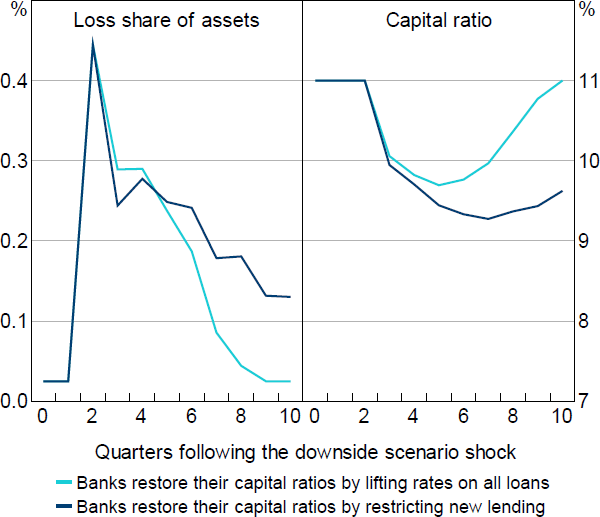
Figure 6 shows the effects that the downside scenario has on the key banking sector variables in BA-MARTIN (loan losses and capital). The figure shows these effects under our baseline assumption that banks reduce credit supply by increasing lending rates on all loans, and our alternative assumption that banks reduce credit supply by restricting new lending. Under both assumptions, the downside scenario decline in GDP, increase in unemployment and fall in housing prices results in a large increase in loan losses. The initial increase in losses is sufficiently large that banks' capital ratios decline by 1–2 percentage points.
As discussed in Section 2.1, increasing interest rates on outstanding loans has a large effect on banks' NIMs, and is therefore a powerful tool for recouping capital when external capital markets cannot be accessed at a cost-effective price. Moreover, by spreading the cost of capital replenishment across new and existing loans, the financial accelerator mechanism is dampened. In Figure 6, this manifests in banks achieving their desired/required speed of capital restoration with lower additional losses than when restricting new lending.

Because we calibrate to match the speed of aggregate capital ratio adjustment implied by the RBA's stress testing framework, the appropriate calibration if banks lift rates on all loans need not be the same as if banks restrict new loans only. We find that, when restricting new loans only, the larger credit supply restrictions required for each bank to achieve a given speed of adjustment lead to such magnified losses that the return of capital ratios to target takes longer (i.e. the aggregate demand externalities are larger). Therefore, approximating the RBA's stress testing framework requires a lower with the ‘restricting new loans only’ assumption. In this section, we set
Importantly, banks' capital ratios remain well above regulatory benchmarks under both credit supply assumptions (both the prudential minimum and regulatory capital buffer (RBA 2021)).
4.2.2 Credit supply response
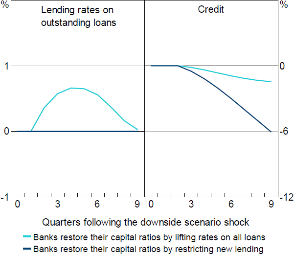
The extent of the credit supply response to the downside scenario in BA-MARTIN can be measured by comparing the path for banks' lending rates and credit to what occurs when the same shocks are applied to MARTIN (Figure 7). When raising rates on all loans, achieving the capital ratio path shown in Figure 6 requires banks to increase their lending rates by 66 basis points. As banks' capital positions improve, banks begin to unwind this lending rate increase. In BA-MARTIN, this path of lending rates results in the level of credit provided to the economy being around 1.5 per cent lower than it would have been without the credit supply restriction.
Importantly, the estimated persistence of the economic variables in MARTIN (which is unchanged in BA-MARTIN) means that this lower level of credit persists well beyond the point that lending rates return to normal, which means that housing prices and economic activity would also be persistently lower. This is important for policymakers, as it means the economic cost of loan losses that are sufficiently high to engender a credit supply restriction lasts well beyond the point at which the credit supply restriction is removed.

This persistent economic cost is much worse if banks decide to constrain new lending to restore their capital ratios.[24] Because a much larger credit supply restriction is required in this situation, credit is 6 per cent below the MARTIN level two years following the crisis. And if banks continue to find external capital raising difficult, this gap would continue to grow.
While examining deviations from MARTIN is the best way to analyse the financial accelerator mechanism, it is important to remember that these reductions in credit supply occur on top of already large reductions in credit demand (due to the original COVID-19 downside scenario shocks). We do not show their combined effect as the downside scenario profile for these variables were not made public with the May 2020 SMP.
4.2.3 Effect on the housing market
Higher interest rates and lower credit growth dampen housing market activity. This dampening effect occurs both as a direct result of increasing the cost/reducing the availability of credit, and indirectly as the reduced housing market activity leads to lower income growth and higher unemployment (which feeds back into the banking sector and housing market).
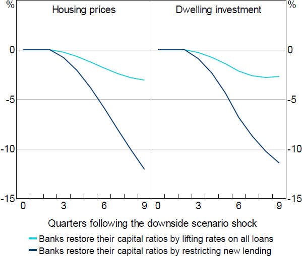
When banks recapitalise by increasing lending rates on all loans, the path of interest rates causes housing prices to decline by an additional 3 per cent after two years (on top of the decline caused by the initial downside scenario shocks), which leads to a similar decline in dwelling investment (Figure 8). When banks restrict new lending, the larger reduction in credit supply results in housing prices and dwelling investment declining by around 12 per cent beyond the fall caused by the initial downside scenario shocks.

4.2.4 Effect on economic activity and unemployment
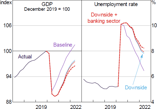
Figure 9 reproduces the scenarios from the May 2020 SMP and adds additional paths to show the amplification caused by the financial accelerator mechanism. When banks spread the credit supply response across all loans, the resulting increase in lending rates (which peaks at a 66 basis point increase) results in a small reduction in economic activity relative to the reduction caused by the COVID-19 shock itself. The level of GDP is around 0.3 per cent lower at the end of the forecast horizon, and unemployment is 0.1 percentage points higher (approximately 16,000 fewer employed people). While this amplification is small relative to the size of the COVID-19 shock, this increase in unemployment is highly persistent, lasting beyond the end of the forecast horizon.
Consistent with the much larger effects on the housing market, if banks restore their capital ratios by restricting new lending, the amplifying effect on economic activity is much larger. GDP would be around 1.3 per cent lower and the unemployment rate would be around 0.4 percentage points higher (approximately 59,000 fewer employed people).

Note: Dashed line indicates when credit supply is restricted on new lending only.
Sources: ABS; Authors' calculations; RBA
It is worth reiterating that, in order to assess how much the banking sector can amplify the macroeconomic effects of crises, we explicitly prevent policy from responding to the amplification. In reality, monetary policy would respond by reducing the cash rate (or via unconventional policies), and it is likely that governments and APRA would also respond. How much monetary policy would need to respond may seem like a simple question – if lending spreads increase by 66 basis points, the effect on lending rates could be offset by reducing the cash rate by the same amount. But this does not account for the fact that the addition of a banking sector to MARTIN changes how monetary policy transmits through the economy, and introduces state-dependence. Assessing this state-dependent policy pass-through is the focus of the next section.
Footnotes
To be clear, banking sector stress was incorporated into the downside scenario using the judgement of RBA staff. Our use of this scenario is to illustrate the new BA-MARTIN mechanisms, not to change the scenario itself. [22]
MARTIN incorporates an endogenous policy response. So our policy assumption in this section should be seen as an explicit aberration for ease of exposition, rather than the way BA-MARTIN typically works. [23]
We do not show the observed increase in lending rates when restricting new loans only because the size of the increase would depend on how the restriction is implemented (e.g. if lending volumes are reduced more for riskier loans, see Section 3.8.3). The reduction in credit is shown as it will not differ between implementations. [24]