RDP 2022-01: MARTIN Gets a Bank Account: Adding a Banking Sector to the RBA's Macroeconometric Model 3. BA-MARTIN in Detail
January 2022
- Download the Paper 1,775KB
In this section, we will detail the banking sector components of BA-MARTIN, and explain how they are derived and calibrated. This section will only detail the model equations to the extent that they aid explanation. Further details of all the equations and parameter calibrations can be found in the Online Appendix.
3.1 Household loan losses
Australian banks provision for losses when they are expected, not just when they are realised. So we define ‘losses’ as the flow of unexpected loan write-offs plus the net change in provisions (as opposed to defining losses as the stock of loan write-offs), and use the term ‘total expected losses’ to refer to the sum of these flows during a given economic deterioration. Both losses and total expected losses are defined as a share of assets.
With provisioning based on expectations, the effect of losses on banks' balance sheets does not depend on when borrowers are actually expected to default on their loans. Therefore, we only need to model how total expected losses respond to economic downturns (as opposed to also needing to model the timing of defaults).
3.1.1 Nonlinear losses
Defining as total expected household loan losses based on the period t extent of the deterioration, household loan losses in period t are defined as:
where the max {.} function ensures that it is only the increase in total expected losses that translates into period t losses (previous increases will have already been provisioned), accounts for the fact that some proportion of household loans are expected to default in each period even without an economic deterioration, and is an exogenous shock that allows us to run scenarios in which losses are smaller/larger than average.
The log of total expected household loan losses is defined as:
where the f (.) function defines how the log of total expected losses is affected by changes in the lagged unemployment gap (to the NAIRU), mortgage rate gap (to the nominal neutral cash rate plus steady state spread) and log housing price gap (to its stochastic trend) – details of how these gap variables are constructed are provided in the Online Appendix.[5]
is calibrated such that, in a downturn equivalent to what APRA assumed in their 2017 stress testing exercise, the sum of quarterly household loan losses equals the total household loan losses in APRA's exercise (APRA 2018).
3.1.2 Micro-simulation model
While APRA's stress testing results provide enough information to calibrate the level of total expected losses, they do not provide sufficient information to identify the potentially nonlinear f (.) function. For this, we use the micro-simulation model designed by Bilston et al (2015) and updated by Kearns et al (2020).
The micro-simulation model takes the distribution of households from the 2017/18 Survey of Income and Housing (SIH), and determines each household's ‘distance to default’ and net initial wealth.[6] Aggregate shocks to interest rates, unemployment and housing prices are then distributed among the households (based on their modelled sensitivity to these shocks) to determine the households that are expected to be unable to continue servicing their mortgage. Expected loan losses are then determined by the amount of debt held by these households minus the post-shock value of their housing collateral and lenders' mortgage insurance (consistent with the double-trigger hypothesis (Bergmann 2020)).
To calibrate the f (.) function from the micro-simulation model, we discretise the continuous gap variables and then run the model for all discrete combinations within the following bounds: and We then use the resulting log expected losses as the dependent variable when estimating the parameters in the following interacted cubic regression (where t subscripts have been removed because the micro-simulation model is static):
The f (.) function is then defined as:
This interacted cubic functional form is sufficiently flexible to capture the majority of the variation in log expected losses, and does a much better job than a linear non-interacted functional form (Figure 2).
Importantly, the slopes of the curves in Figure 2 are marginal effects. To explain the ‘total effect’ using an example, the total effect of an increase in unemployment on losses encompasses both the marginal effect and the indirect effects that occur via the resulting changes in housing prices and mortgage rates. The high degree of estimated nonlinearity also means that the starting point matters; for example, the marginal benefit of a decrease in the mortgage rate is larger when the starting point for total expected losses is higher.
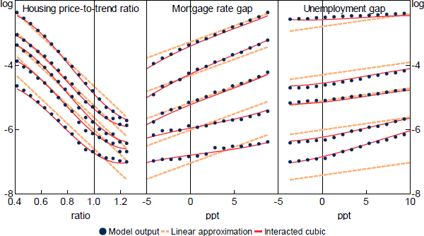
Note: Quantiles determined by varying the other variables.
3.1.2.1 Compromises
Ideally, the model used to calibrate the f (.) function would estimate total expected losses based on the expected size and duration of a given downturn. Unfortunately, the micro-simulation model we use is only able to estimate expected losses based on the expected size of the downturn (as it is a static model based on a cross-section of data). So we will likely overestimate the effect of short downturns and underestimate the impact of protracted downturns.
Moreover, MARTIN does not contain explicit equations for expectations. So we further compromise by assuming banks provision based on the contemporaneous extent of the deterioration; provisioning for losses will therefore be slower in our model than in reality.
With the micro-simulation model being much more detailed than our three-variable f (.) function, there are multiple determinants of expected losses that we (at best) implicitly capture via their relationships with our three included variables. For example, the influence of households' loan-to-valuation ratios (LVRs) and prepayment buffers at their 2017/18 surveyed levels is implicitly captured within the modelled relationships between the three included variables and expected losses (e.g. lower LVRs would mute the marginal effect of housing price declines on losses). However, this static and implicit capturing of average LVRs and prepayment buffers means any beneficial effect slower credit growth might have on improving resilience to future shocks will not be modelled (e.g. Schularick and Taylor 2012).
Endogenising households' resilience would be a fruitful avenue for future model development. In the meantime, to ensure households' resilience is at least exogenously updated, we recommend that Equation (2) be re-calibrated with each new SIH wave, and that users of this model be aware that any non-modelled changes that have occurred between the survey and the point of the shock will not be captured.
3.2 Total loan losses
We do not currently model losses on business loans, and simply assume business loan losses move proportionately with housing loan losses. This is obviously unrealistic. But we are not currently able to include a model for business loan losses as MARTIN does not currently have equations for business credit growth or commercial property prices, and the RBA is currently reviewing its business loan stress testing framework.
So that a model for business loan losses can be easily incorporated once the necessary components have been developed, we set business loan losses equal to some calibrated multiple of household loan losses:
And define total losses as:
where and have the business loan equivalent definitions of Equation (1), and is the household share of banks' outstanding loans (estimated from APRA data). Once an equation for business loan losses has been developed, the only change that needs to be made is to substitute this new equation for Equation (5).
In the meantime, is calibrated such that, in a downturn equivalent to what APRA assumed in their 2017 stress testing exercise, the sum of quarterly losses equals the total loan losses in APRA's exercise (APRA 2018).
3.3 Risk-weighted assets
For capital adequacy purposes, assets are risk weighted; if banks have riskier assets on their balance sheets, they need more capital to meet regulatory capital requirements. Risk weights are determined by a combination of APRA and the banks' perceptions of default probabilities and probable losses (APRA 2020). They therefore tend to co-move with losses but stay elevated longer than losses (RBA 2017).[7] To capture this extended cyclicality in a simple way, we model risk weights as an autoregression nonlinearly shocked by losses:
In reality, risk weights differ by asset class. Since we don't incorporate detailed asset mix data into BA-MARTIN, the risk-weight multiplier we use ( wt ) is the weighted-average value such that when multiplied by total assets at the beginning of the next period ( At+1 ) the resulting value equals the value of the banking system's risk-weighted assets.
With , an increase in losses causes an increase in wt; risk weights will continue to grow as long as losses are larger than the steady-state level . Once losses fall back to their steady-state level, the will cause the risk-weight multiplier to slowly move back to its steady state of (higher values of increase the speed of adjustment).
We calibrate based on banks' average risk weights during 2019. We calibrate and such that, when we input the losses from APRA's 2017 stress tests, Equation (7) produces a path of risk weights that approximately replicates the APRA stress test path.
3.4 Debt funding costs
Australian banks' high-interest deposit and non-deposit debt funding spreads have historically been determined more by liquidity/risk conditions in global funding markets than by domestic economic conditions (Brassil et al 2018). But increases in credit risk would increase banks' cost of debt funding. When the cash rate is sufficiently far above zero, we model these spreads as an exogenous random walk (to reflect the exogenous global markets and any other exogenous changes to these spreads) plus a term that increases with credit risk.
As in Major (2016), we model increases in credit risk as being linearly related to deteriorations in banks' capital adequacy. Using a panel regression of bond market spreads on capital ratios, Major found that a 1 percentage point fall in a bank's capital adequacy ratio is expected to increase its debt funding costs by 10 basis points; we calibrate our model to match this estimate.[8]
3.4.1 Zero lower bound
Retail deposit rates tend to have a lower bound around zero – due to the possibility of holding physical currency instead. Some bank deposits always pay near-zero interest. The lower bound does not matter much for these non-interest bearing accounts because banks hedge the fixed interest rate risk of these deposits using a ‘replicating portfolio’ hedge (Brassil et al 2018).
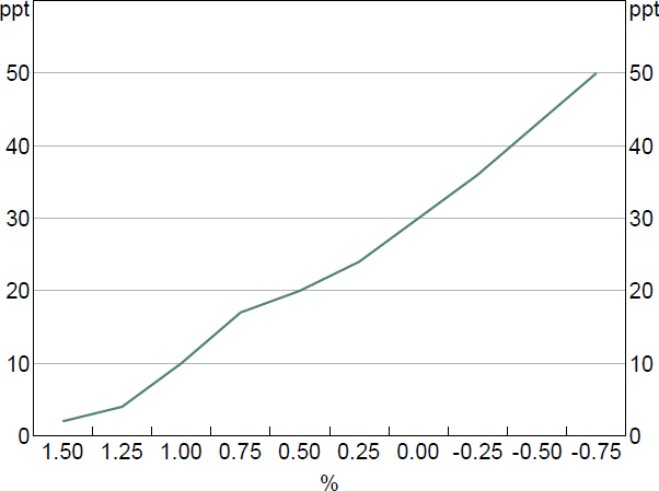
For deposit accounts that typically pay an above-zero rate of interest, this lower bound would bind only after the cash rate falls below a certain level. As it is costly to effectively hedge against an occasionally binding lower bound, banks remain exposed to this funding risk. The result is that banks' costs of funding fall by less than the cash rate once the cash rate moves below a certain level; in other words, the spread between the cash rate and banks' cost of funding increases as the cash rate falls.
We use the information in Garner and Suthakar (2021) and discussions with RBA staff to model the increasing share of deposits at the lower bound as the cash rate falls below 1.5 per cent (Figure 3). How we incorporate this information into the BA-MARTIN equation for debt funding costs ( rD,t ) is explained in the Online Appendix. And the effect of the lower bound on monetary policy pass-through is explored in Section 5.[9]
3.5 Interest income
The lending spreads banks charge above their costs of debt funding have historically been unrelated to the level of interest rates (see Graph 13 in Garner and Suthakar (2021)). So we assume that when banks' capital ratios are at their desired level, they charge borrowers an exogenous spread above their costs of debt funding. We call these exogenous spreads ‘unconstrained lending spreads’, and model them as random walks – the unconstrained business spread is sB,t and the unconstrained housing spread is sM,t .[10]
When capital ratios fall below banks' desired levels, banks increase the spreads they charge borrowers above these unconstrained spreads. How banks respond to these capital deteriorations is explained in Section 3.8.
3.6 Profits (return on assets)
Banks' profits comprise their net non-interest income plus net interest income, less their loan losses (all after tax). For our purposes, it is sufficient to define banks' return on assets (ROA = profits / assets) rather than their profits.
Banks' net interest margins (net interest income as a share of assets) equal their average lending rates ( rA,t ), minus their average debt funding costs ( rD,t ) times their debt-to-assets ratio (equivalently defined as one minus their capital-to-assets ratio ( Et / At )). Using this definition and the previously defined losses variable ( Lt ), banks' return on assets ( ROAt ) is defined as:
where is one minus the corporate tax rate, represents banks' net non-interest income as a share of assets (assumed constant for simplicity), and banks' NIMs are divided by 400 because the model is quarterly and MARTIN interest rates are in annual percentage units.[11]
The NIM can be equivalently written as the net interest spread ( rA,t – rD,t ) plus the product of debt funding costs and the capital ratio. The net interest spread equals the weighted average of the unconstrained mortgage and business lending spreads plus any endogenous increase in spreads that results from banks wanting to improve their capital ratios following a deterioration (defined as ).[12] Substituting these definitions into the first line of Equation (8) is how we get to the second line.
3.7 Capital adequacy ratio
Using the asset risk-weight multiplier ( wt ), the capital-to-risk-weighted assets ratio at the beginning of period . The change in this ratio can be decomposed as (this decomposition is the discrete-time version of the total derivative):
We use the existing MARTIN equation for household credit growth (Equation (19) in the Online Appendix of Ballantyne et al (2019)) as a proxy for all credit growth (since MARTIN does not have a business credit growth equation). MARTIN's household credit growth equation can be written as a function of the contemporaneous mortgage rate and other endogenous and exogenous variables:
where Xt is a vector of the ‘other’ endogenous and exogenous variables in the household credit growth equation (these variables are all determined in period t or earlier, and include lags of the mortgage rate is the MARTIN-estimated contemporaneous effect of the mortgage rate on household credit growth, and B is a vector of coefficients defined in MARTIN.[13]
The change in capital / assets equals banks' return on assets ( ROAt ) plus new raisings of capital from external sources as a share of assets ( ENew,t / At ) minus the share of dividend payments ( Dt / At ).
Substituting all of the above into Equation (9) gives the following approximation:
Equation (11) is an approximation because we replace the et+1 interaction with credit growth (in Equation (9)), with et. This approximation ensures that the right-hand side of Equation (11) is a function of variables from period t or earlier ( is a function of lagged variables).[14]
3.7.1 State dependence
There are three as yet undefined endogenous variables in Equation (11): banks' new raisings of capital from external sources ( ENew,t ), their dividend payments ( Dt ), and within ROAt and is how banks increase their lending spreads in response to a capital deterioration . How banks set will be explained in Section 3.8. How banks set ENew,t and Dt depends on the state of the economy.
We assume that, when banks' capital adequacy ratios fall below target (i.e. when losses are sufficiently high), the cost of raising new capital would be sufficiently prohibitive that banks would not choose this option. We further assume that with capital adequacy below target, banks would retain as much of their earnings as possible – so banks would not pay dividends. Therefore, in what we call the ‘stressed state’, ENew,t = Dt = 0.
Outside of the stressed state, in what we call the ‘unconstrained state’, we assume banks are able to access external capital markets, and do so such that any demand-driven credit growth has no effect on their capital adequacy . In other words, external capital markets are accessed to fund new lending.[15]
Banks spend most of their time in the unconstrained state. And, as noted above, entry into the stressed state occurs when losses push banks' capital adequacy ratios below target. But it's not necessarily the case that the cost of raising new capital remains prohibitive for the entire time capital ratios remain below target (i.e. banks may re-enter the unconstrained state before their capital adequacy ratios return to their target levels). To capture this flexibility in our model, we allow the user to set the number of periods for which the stressed state lasts (see the Online Appendix for details).
We assume dividends remain at zero while capital adequacy is below target. Once capital returns to target, we assume dividends are set such that whenever Equation (11) would otherwise be positive. In other words, banks pay out excess profits as dividends.
It is worth noting that the lack of recent periods of extreme banking stress in Australia make it difficult to determine exactly how banks would respond in such a scenario. The assumptions we make around external capital raisings and dividend payments, which are consistent with the RBA's stress testing framework (RBA 2017), should therefore be seen more as prudent modelling choices that ensure we do not underestimate the financial accelerator effect, rather than exactly how banks would behave.
3.8 Credit supply
Consistent with the RBA's stress testing framework (RBA 2017), we assume banks only restrict credit supply in response to a capital shortfall. If we define banks' target for their capital adequacy ratio as , then if banks do not restrict credit supply their capital shortfall in period t +1 can be defined as:
where is defined as the value of (from Equation (11)) given the period ( t ), value of the credit supply response , and state of the economy (St).[16]
Now suppose banks restrict credit supply such that their capital shortfall in period t +1 is smaller than suggested by Equation (12):
where can be interpreted as the desired/required speed at which the capital adequacy ratio returns to target. If , Equation (13) simplifies to ; that is, there is no credit supply response and the speed at which the capital adequacy ratio returns to target is determined by P(t,0,St). If , credit supply is sufficiently restricted such that the capital ratio is returned to target within one period . If , credit supply is restricted such that the capital ratio is returned to target faster than P(t,0,St), but at a rate that allows a persistent capital shortfall.
By solving for the value of such that banks' capital ratios return to target at the speed defined in Equation (13) (i.e. setting the unique credit supply reduction that satisfies this equality is:[17]
In other words, the speed of adjustment uniquely determines how much banks increase their lending rates in response to a deterioration in capital adequacy. And these endogenously set lending rates combine with MARTIN's credit growth equation (Equation (10)) to determine the resulting rate of credit growth in the economy.
3.8.1 Calibrating the speed of adjustment
We calibrate so that banks return their capital ratios to target with a speed of adjustment that broadly matches the speed implied by the RBA's stress testing framework. In their framework, capital ratios return to target around 2–3 years from the downturn. So we approximate this by setting (Figure 4).
The amplification through the banking sector is clear in Figure 4. Following the initial shock, higher credit supply responsiveness leads to higher household and business lending rates and a faster return of capital to target. But the higher lending rates increase repayment burdens, reduce housing prices and investment, and increase unemployment, leading to higher losses. These losses further increase lending rates (relative to the counterfactual), and so on.[18]
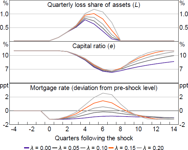
Notes: The shock is consistent with the shock used by APRA in their 2017 stress testing exercise (APRA 2018) – a 35 per cent fall in housing prices and unemployment increasing 5 percentage points. The cash rate is held constant following the initial policy response to the shock (125 basis points, as in the stress testing exercise).
3.8.2 Banks' choices have aggregate demand externalities
When determining how banks set their credit supply responses, it's important to differentiate between the variables each bank determines solely through their own choices, and the variables that depend on the choices made by all banks. This is because, even if all banks make the same choices in equilibrium, in a competitive system each bank treats the choices made by other banks as independent of their choice.[19] The result is that banks make different choices to what a monopolist would choose, thereby causing what is known as an ‘aggregate demand externality’.
In our model, these externalities amplify the financial accelerator mechanism. While each bank accounts for the effect their interest rate decision has on their NIM and credit growth, losses and risk weights are mostly determined by aggregate variables – such as housing prices and unemployment – and therefore depend on the decisions made by all banks.[20] Given that credit supply reductions amplify losses, these externalities lead to larger losses than if banks internalised the effects their combined decisions had on losses.
Figure 5 shows the effect of these externalities on the speed at which capital ratios return to target. The maroon bars show the effect of banks' credit supply decisions on NIMs and credit growth (i.e. the effects banks internalise), while the blue and orange bars show the effects these credit supply decisions have on losses and risk weights. During the peak of the stressed period, these extra losses and risk weights work against the NIM and credit growth changes, such that banks' capital ratios do not actually change much with the reduced credit supply. It is only when losses normalise that capital ratios increase at a noticeably faster speed.

To be absolutely clear, each bank's credit supply reduction still improves its capital ratio at the speed required by Equation (13). To explain why, suppose we looked at the Figure 5 equivalent for an individual bank. If this bank did not reduce its credit supply but all other banks did, then it is only the maroon bars that would be removed, the blue and orange bars would remain; the size of the maroon bar in period t equals the extra speed of adjustment required by Equation (13) .
3.8.3 Credit supply reduction affects new loans only
With this alternative assumption, banks' credit supply reductions have only marginal direct effects on their NIMs (as NIMs are determined by outstanding loans). Therefore, banks are only able to directly increase their capital ratio by reducing credit growth (i.e. through the denominator of the capital ratio). With the credit supply reduction working through the denominator only, achieving the same increase in the capital ratio requires a much larger reduction in credit supply, resulting in a much larger financial accelerator mechanism than with our baseline assumption.
Only minor changes to BA-MARTIN are required to implement this alternative assumption. This is because the original MARTIN relationship between household credit growth and lending rates remains unchanged (as it is determined by the lending rates available for new loans). With this credit growth-lending rates relationship unchanged, the endogenous credit supply reduction can still be implemented in BA-MARTIN via , but the interpretation of may become more nuanced (explained in more detail below). The changes required to BA-MARTIN are:
The direct effect of interest rates on losses occurs because increases in the interest rates of outstanding loans increase households' interest burdens and therefore increase the proportion of households unable to continue making payments. With only affecting new loans in this scenario, it is the mortgage rate gap without the credit supply reduction that enters the losses equation (Equation (15)).[21] NIMs are also determined by outstanding loans, so also needs to be removed from banks' return on assets (Equation (16) defines return on assets after this removal).
With each bank's credit supply reductions now working through credit growth only, the unique credit supply response that achieves the desired/required speed of adjustment is Equation (17); this response is always larger than Equation (14).
The interpretation of in this new-loans-only scenario is ‘the weighted average increase in lending rates paid by new borrowers, with constant weights’. The constant weights part of this interpretation is important if, for example, banks reduce lending volumes more for riskier loans (i.e. lending standards are tightened). In this case, even though each borrower would be paying more for their loan, the proportion of new borrowers would shift towards those with lower risk; so average lending rates with shifting weights need not increase. To achieve the correct credit supply reduction in BA-MARTIN, must reflect the average increased borrowing costs at the previous weights.
Footnotes
Lags are used to avoid introducing circular references that would require us to adapt multiple existing MARTIN equations. Intuitively, the gap variables are designed to capture the fact that losses depend on how these variables evolve relative to long-run expectations. [5]
Distance to default is defined as a household's post-tax income (including transfers) after rent and loan payments, minus the Household Expenditure Measure (developed by the Melbourne Institute, and used as a minimum consumption benchmark). A household is assumed to be unable to service its mortgage once successive periods of negative ‘distance’ more than offset the household's liquid assets (e.g. balances in offset/redraw accounts). [6]
During COVID-19, for example, the major banks estimated that in some scenarios these procyclical increases in risk weights could have subtracted 70 to 180 basis points from their capital ratios (RBA 2020b). [7]
The Major (2016) estimates are derived from a linear model over a period during which the credit quality of the Australian banking sector remained high; so we likely underestimate the change in debt funding costs that would occur during an extreme stress scenario. [8]
In some jurisdictions, banks have increased fees to offset the deposit lower bound (Hack and Nicholls 2021). There is no evidence of this occurring in Australia at this stage (Sparks and Garner 2021). [9]
MARTIN does not incorporate interest rates for non-housing personal loans. Instead, the housing spread is used as a proxy for the spread on all household loans (more than 90 per cent of household loans are for housing). [10]
Although banks' net non-interest income is not constant, between 2004 and 2017 it had a constant mean (relative to assets) and exhibited little persistence (see Figure 11 in Brassil et al (2018)). [11]
We assume the credit supply response is imposed equally on household and business loans. [12]
will not simply equal the coefficient of the nominal mortgage rate in the household credit growth equation. This is because the real mortgage rate also appears in the credit growth equation; is time-varying because the difference between the nominal and real mortgage rates depends on the rate of inflation. [13]
This approximation means the approximate value of will equal the true value times . Therefore, as long as quarterly credit growth is close to zero, this approximation will not deviate too far from the true value. [14]
We assume banks only offset the demand-driven credit growth, which is defined as credit growth excluding any credit supply responses , since reducing external capital raisings to offset credit supply reductions would be counterproductive. [15]
zt has a subscript t because all determinants of the period t +1 capital shortfall are known in period t. [16]
Given that we are using MARTIN's household credit growth equation as a proxy for total credit growth, for the purposes of determining we assume the relevant interest rate for credit growth is rA,t (i.e. in Equation (10) we replace rM,t with rA,t for the purposes of determining ). [17]
Even with , the mortgage spread to the cash rate increases in Figure 4 (i.e. the purple line rises despite a constant cash rate). This is due to the effect of the capital deterioration on debt funding costs. [18]
With four major banks, each of the majors would likely account for the effects of their decisions on aggregate variables. So treating the Australian system as perfectly competitive is a simplification. [19]
Solving for the value of that satisfies Equation (13) is approximate to solving for each bank's infinite-horizon optimal credit supply (for a given ). This is because the effects that banks internalise (NIMs and credit growth) are close to independent of past values of z* (the small dependency is shown in the ‘Other’ bar in Figure 5), while the effects they do not internalise (losses and risk weights) and that appear in Equation (13) are independent of . [20]
Importantly, losses will still increase indirectly via the lower housing prices and higher unemployment caused by the credit supply reduction. [21]