RDP 2021-09: Is the Phillips Curve Still a Curve? Evidence from the Regions 2. Background on the Phillips Curve and the RBA's Modelling Approach
September 2021
- Download the Paper 1,707KB
2.1 The Phillips curve
The intuition underlying the Phillips curve is that ‘[w]hen the demand for labour is high and there are very few unemployed we should expect employers to bid wages rates up quite rapidly’ (Phillips 1958, p 283), and firms to raise prices.
Although much of the Phillips curve literature relates to the relationship between price inflation and unemployment, similar intuition applies to the wages growth–unemployment relationship. Notably, both the RBA and Australian Treasury use versions of a Phillips curve as their preferred models for forecasting nominal wages growth. In this and the following section we largely deal with wage and price Phillips curves interchangeably. However, from Section 4 on we limit our empirical analysis to the wage Phillips curve, which is the relationship we are most interested in.[3]
Since Phillips (1958), a vast amount of theoretical work has built on and formalised this basic intuition. Milton Friedman's (1968) expectations-augmented Phillips curve is:
where is inflation, is expected inflation, ut is unemployment, is the non-accelerating inflation rate of unemployment (NAIRU), and et is an error term.[4],[5] The difference between ut and is the ‘unemployment gap’. This basic framework was also extended to include supply shocks by Gordon (1982). Because neither expected inflation nor the NAIRU can be directly measured, they need to be estimated.[6]
An equation like the expectations-augmented Phillips curve also appears in many New Keynesian DSGE models, and is called the New Keynesian Phillips curve. In these macroeconomic models with sticky prices, there is a positive relationship between the rate of inflation and the level of demand, and therefore a negative relationship between the rate of inflation and the rate of unemployment.
2.2 Sources of nonlinearity
The Phillips curve above (Equation (1)) assumes the relationship between the unemployment gap and inflation is linear: a 1 percentage point increase in the unemployment gap has the same effect on inflation when the labour market is tight as it does when the labour market has plenty of spare capacity. However, Phillips (1958) himself argued that the relationship between unemployment and wages growth is likely ‘highly non-linear’ as ‘workers are reluctant to offer their services at less than the prevailing rates when the demand for labour is low and unemployment is high so that wage rates fall only very slowly’. This explanation relates to the notion of downward nominal wage rigidity - that firms are either unwilling or unable cut nominal wages. During recessions these rigidities become more binding and labour market adjustment disproportionately occurs via higher unemployment rather than via lower wages. During expansions, where rigidities bind less, more of the adjustment can occur via wages.[7] This is an important argument for a nonlinear (convex) Phillips curve, especially in a low inflation environment.
Evidence from job-level microdata up until 2018 suggests that downward nominal wage rigidity is a binding constraint for Australian employers. A histogram of job-level annual wages growth outcomes from the wage price index (WPI) shows clear evidence of a scarcity of wage cuts and an abundance of wage freezes, consistent with downward nominal wage rigidity (Figure 2). In fact, only 1 per cent of all jobs experience a wage cut in any given year, compared with around 22 per cent experiencing a wage freeze.[8]
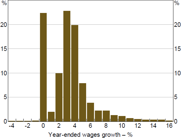
Sources: ABS (job-level wage price index microdata); Authors' calculations
Another common explanation for a convex Phillips curve is the presence of capacity constraints. This argument supposes that firms find it difficult to increase their production capacity in the short run. So, when an economy experiences a strong rise in demand, more firms will run up against capacity constraints which will push up wages and prices. Further, inflation becomes increasingly sensitive to demand; each additional increase in demand leads to ever-increasing rises in inflation. Debelle and Laxton (1997), Debelle and Vickery (1997) and Kumar and Orrenius (2016) suggest that these ‘bottlenecks’ arise when the unemployment rate falls below the NAIRU or natural rate of unemployment.[9]
Other explanations for a convex Phillips curve include menu costs and relative prices (Ball and Mankiw 1994) and efficiency wages (Shapiro and Stiglitz 1984); see Dupasquier and Ricketts (1998) for a summary of these arguments. Standard models of the labour market also imply such nonlinearity (Petrosky-Nadeau and Zhang 2017).[10]
2.3 The RBA's modelling approach
This nonlinearity in the inflation–unemployment trade-off was explicitly incorporated into the RBA's wage and price inflation models in the late 1990s, following a research discussion paper by Debelle and Vickery (1997). Prior to that, the RBA's Phillips curves were estimated in a linear framework; that is, assuming that the effect on inflation of each percentage point change in unemployment is the same regardless of the level of unemployment.
From an empirical standpoint, Debelle and Laxton (1997) and Debelle and Vickery (1997) argued that a nonlinear relationship between inflation and the unemployment gap provided a better fit to the national time series data for the United Kingdom, the United States, Canada and Australia. The equation they estimated essentially replaced the linear unemployment gap in Equation (1), , with the unemployment gap relative to the level of unemployment:
This specification implies a short-run slope equal to:
In this specification, a change in the unemployment rate has a different effect on inflation depending on both the current level of the unemployment rate and the NAIRU. Since Debelle and Vickery (1997), the RBA's workhorse wage and price Phillips curve models for policy analysis and forecasting have assumed this nonlinear relationship between inflation and the unemployment gap (Cassidy et al 2019; Ballantyne et al 2019).[11] In practice, the RBA's current models also control for other determinants of wage and price inflation, including lagged inflation and controls for supply shocks. In this paper, our discussion of the RBA's aggregate Phillips curve models focuses on the set of single-equation Phillips curve models used in constructing the RBA's central forecasts for wage and price inflation. The specifications of these models are set out in Appendix A (for wage inflation) and Cassidy et al (2019) (for price inflation). In practice, the RBA also maintains a full-system economic model for risk and scenario analysis, which adopts a similar nonlinear unemployment gap in its wages equation (Ballantyne et al 2019). Recent analysis, including the forecast scenarios for price inflation presented in RBA (2021b), has also incorporated a nonlinear unemployment gap in the inflation equation.
The functional form used in the RBA's current forecasting models for wages growth and underlying price inflation implies a high degree of nonlinearity in the Phillips curve (Figure 3). The estimates of from the RBA's model of price inflation are –2.74 and –1.90 for wage inflation. If we substitute these estimates into the expression for the slope of the Phillips curve, along with the current level of the unemployment rate (ut = 4.6 per cent) and an assumption for the NAIRU ( = 4.5 per cent), it implies that the slope of the price Phillips curve (at tangency) is –0.58, that is, a 1 percentage point change in the unemployment rate from its current level would lead to a 0.51 percentage points change in inflation. For wages growth, the slope is slightly flatter at –0.40. If we instead assumed Australia had an unemployment rate of 4 per cent, as currently forecast for the end of 2023, the RBA's preferred models imply that the Phillips curve would be 30 per cent steeper (holding and fixed).[12]
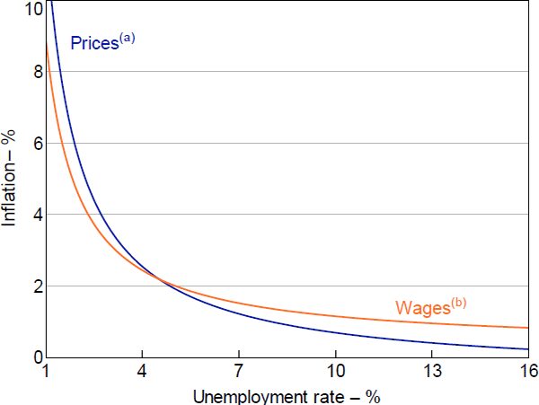
Notes:
Short run; annualised; assumes NAIRU at 4.5 per cent; the vertical position of the curves is set by assuming that when the unemployment rate equals 4.5 per cent, both wage and price inflation equal 2.2 per cent
(a) Trimmed mean consumer price index inflation; estimated over 1993:Q2–2019:Q4
(b) Private sector wage price index inflation; estimated over 1998:Q1–2019:Q4
Sources: ABS; Authors' calculations; RBA
As a consequence of this nonlinearity, the RBA's models imply that the responsiveness of wage and price inflation to a percentage point change in the unemployment rate has changed over time as the economy has moved along the Phillips curve (Figure 4).[13] Based on the estimated wage Phillips curve coefficients, inflation was increasingly responsive to changes in unemployment during the 1990s and during the resources boom, as the unemployment gap steadily declined and the economy moved to a steeper part of the curve. This gradual tightening in the labour market meant that by 2008, the economy was at a point on the wage Phillips curve that was seven times as steep as it was in the aftermath of the early 1990s recession. This trajectory reversed with the GFC, as the rise in spare capacity moved Australia to a much flatter segment of the Phillips curve.
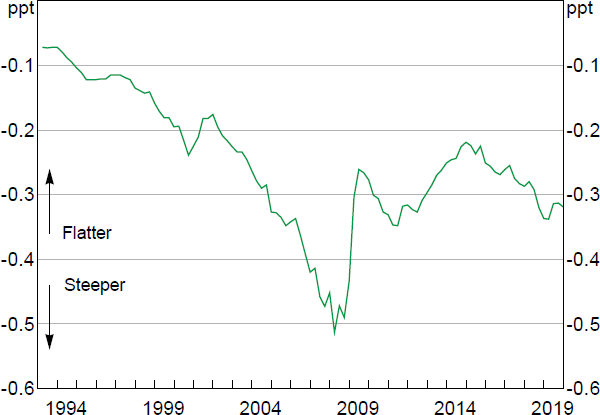
Notes: Short run; annualised; as implied by the RBA's wage Phillips curve model; assumes the NAIRU is fixed at 4.5 per cent
Sources: ABS; Authors' calculations
Footnotes
Data limitations also dictate our focus on wage Phillips curves – high-quality price data are not available in Australia at the local labour market level. [3]
The NAIRU is the unemployment rate consistent with inflation being equal to long-run inflation expectations. It is not observable and has to be estimated. The RBA's current approach is to update the NAIRU estimate based on incoming data on unemployment, labour costs and inflation using a Phillips curve framework that treats the NAIRU as an unobserved variable (Cusbert 2017). [4]
Since Friedman (1968), theorists have derived equations that are broadly similar to Equation (1) from models in which price setters have incomplete information (e.g. Lucas 1973; Mankiw and Reis 2002) or nominal prices are sticky (e.g. Roberts 1995). [5]
See Cusbert (2017) for a discussion in the Australian context. [6]
Theoretical models predict that downward nominal wage rigidity can lead to a nonlinear (convex) relationship between inflation and unemployment in both the long run (Akerlof et al 1996) and short run (Daly and Hobijn 2013). Daly and Hobijn also argue that these rigidities cause recessions to result in substantial pent-up wage deflation. [7]
Using job-level data from a private sector survey, Dwyer and Leong (2000) find strong evidence of downward nominal wage rigidity in Australia in the period 1987–99. Charlton (2003) finds downward rigidity in Australian base wages. [8]
See Dupasquier and Ricketts (1998) for a discussion of capacity constraint-driven Phillips curve convexity and its implications for monetary policy. [9]
Although the majority of papers deal with a convex Phillips curve, one branch of the literature (e.g. Stiglitz 1997) posits that a concave Phillips curve could arise due to asymmetric price adjustment under imperfect competition. The idea is that under monopolistic competition, firms might lower prices to undercut rivals when the economy is slowing (and unemployment is high), but will be reluctant to raise prices when demand is strong (and unemployment is low). [10]
The Australian Treasury also uses a nonlinear Phillips curve specification in its medium-term economic projection framework (e.g. Chua and Robinson 2018) and to estimate the NAIRU (Ruberl et al 2021). [11]
These calculations pertain to the slope of the short-run Phillips curve. The slope of the long-run price Phillips curve can be obtained by multiplying the short-run slope estimates by a scaling factor of 1.25 – the result of dividing the short-run slope of the curve by 1 minus the coefficient on lagged inflation from Cassidy et al (2019). In the case of the wage Phillips curve, the appropriate scaling factor is closer to 1.5 (see Appendix A). [12]
Figure 4 presents the RBA aggregate model-implied slope of the wage Phillips curve, assuming the NAIRU is fixed at 4.5 per cent. Allowing the NAIRU to vary over time (as it does in practice in the RBA's Phillips curve models) yields a qualitatively similar slope profile, although the magnitudes are a little larger, particularly over the first half of the time period, reflecting the drift lower in the RBA's central estimate of the NAIRU over the past two decades (see Figures A1 and A2). [13]