RDP 2021-09: Is the Phillips Curve Still a Curve? Evidence from the Regions 6. Allowing for Kinks in the Phillips Curve
September 2021
- Download the Paper 1,707KB
6.1 A single kink
The linear specification provides a useful benchmark. However, as we will show, the assumption of linearity is strongly rejected by the data (as might be expected based on Figure 6). The simplest way of allowing the slope of the Phillips curve to vary with the level of unemployment is to use a linear spline. This lets us include a kink in the Phillips curve at some threshold unemployment rate, . To estimate a linear spline with a single kink, we only need to add a single new variable to the linear specification,
The additional term allows the slope of the Phillips curve to differ when uit is above or below the kink point, (which is specified before estimation). The slope of the curve below the kink point is given by and the slope of the curve above the kink point is given by . The Phillips curve is downward sloping and convex if and . The key decision is where to place the kink point. Guided by the visual relationship that is apparent in Figure 6, our starting point is to assume that the kink in the Phillips curve (if any) will occur at an unemployment rate of 4 per cent.
The first three columns of Table 2 show results from estimating Equation (4) with set equal to 4 per cent. The three specifications are labelled (B), (C) and (D) and are the same as specifications (B), (C) and (D) in Table 1, albeit after adding the linear spline term to the equation.
Our estimates of and in specification (B) are –0.73 and 0.56, respectively (both statistically significant at the 1 per cent level). This suggests that a 1 percentage point fall in the unemployment rate is associated with an increase in wages growth of 0.73 percentage points when the unemployment rate is below 4 per cent, and 0.17 percentage points when it is above 4 per cent. The statistically significant coefficient estimate for means that we can reject the null hypothesis that the Phillips curve is a straight line.
| Linear spline with single kink | Restricted cubic spline with three kinks | ||||||
|---|---|---|---|---|---|---|---|
| (B) | (C) | (D) | (B) | (C) | (D) | ||
| Unemployment rate | −0.734*** (0.206) |
−0.774*** (0.213) |
−0.733*** (0.215) |
−0.484*** (0.106) |
−0.515*** (0.109) |
−0.512*** (0.102) |
|
| Linear spline term | 0.561*** (0.200) |
0.512** (0.203) |
0.579*** (0.219) |
||||
| Restricted cubic spline term | 0.300*** (0.087) |
0.239*** (0.088) |
0.357*** (0.088) |
||||
| Lagged wages growth | 0.236*** (0.040) |
0.186*** (0.038) |
0.238*** (0.040) |
0.239*** (0.039) |
0.188*** (0.038) |
0.241*** (0.039) |
|
| Unemployment rate × post_2012 | −0.095 (0.265) |
0.097 (0.082) |
|||||
| Linear spline term × post_2012 | 0.048 (0.303) |
||||||
| Restricted cubic spline term × post_2012 | −0.183 (0.111) |
||||||
| Region fixed effects | Yes | Yes | Yes | Yes | Yes | Yes | |
| Time fixed effects | Yes | Yes | Yes | Yes | Yes | Yes | |
| Region-specific trends | No | Yes | No | No | Yes | No | |
| Observations | 5,639 | 5,639 | 5,639 | 5,639 | 5,639 | 5,639 | |
|
Notes: Standard errors (in parentheses) are clustered by region; ***, **, and * denote statistical significance at the 1, 5, and 10 per cent levels, respectively; estimation is done using the Arellano-Bond estimator, and weighted by the number of employees in each region Sources: ABS; Authors' calculations; National Skills Commission |
|||||||
Again, the estimated Phillips curve is slightly steeper – both above and below the kink point – when we allow for region-specific time trends in column (C). And once again, there is no evidence that the slope (or convexity) of the Phillips curve changed after 2012 (specification in column D). In all three specifications, we reject the null hypothesis of linearity at the 1 per cent level of significance. The estimated Phillips curve is convex to the origin, consistent with the assumption in the RBA's aggregate workhorse models following Debelle and Vickery (1997).
6.2 Allowing more curvature
A single-kinked spline may not be flexible enough to capture the curvature of the Phillips curve. To allow for more curvature, we also estimate the wage Phillips curve using a linear spline with three kinks: at unemployment rates of 4 per cent, 5.5 per cent and 7.5 per cent. The locations of these kink points are consistent with similar research for the United States (Leduc, Marti and Wilson 2019; Hooper et al 2019), and correspond to the 23rd, 53rd and 80th percentiles of the distribution of observed unemployment rates in our sample. We plot the estimated Phillips curve using this triple-kinked specification in Figure 7.[35] The estimated Phillips curve is convex to the origin, and the null hypothesis of linearity is rejected at the 1 per cent level of significance (based on a joint test of significance of all three spline terms).
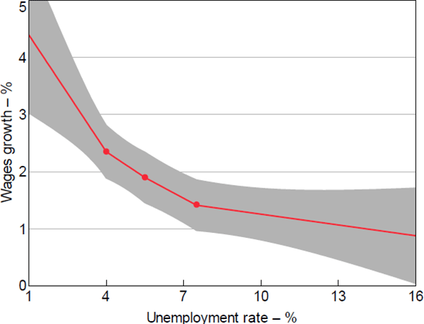
Notes: 95 per cent confidence intervals estimated using the Delta method; dots denote kinks at 4.0, 5.5 and 7.5 per cent
Sources: ABS; Authors' calculations; National Skills Commission
In Figure 7, the slope of the Phillips curve at unemployment rates below 4 per cent is –0.68 (p-value = 0.002), which is only slightly smaller than our estimates at similar levels of unemployment in the single-kink specification. The slope is flatter at –0.30 for unemployment rates between 4 per cent and 5.5 per cent, and flatter still at –0.24 for unemployment rates between 5.5 per cent and 7.5 per cent. When the unemployment rate exceeds 7.5 per cent, the Phillips curve is almost completely flat; the point estimate of –0.06 is not statistically different from zero (p-value = 0.200).
It is important not to get too hung up on the vertical position of the curve in Figure 7, as this is not something that is pinned down by our modelling framework. For example, the figure should not be read as indicating that wages growth will be 2.2 per cent at an unemployment rate of 4.5 per cent. The vertical intercept of the curve in the figure (and similar figures below) is purely illustrative and based on an assumption that wages growth will equal 2.2 per cent when the unemployment rate is 4.5 per cent. In reality, the vertical position of the curve in the wages growth–unemployment space will depend on the NAIRU, inflation expectations and trend productivity growth. While our approach controls for the confounding effects of these variables, it does not estimate them. In other words, our model tells you about the slope and curvature of the Phillips curve, but it does not tell you everything you need in order to make a wages growth forecast based on the unemployment rate. The Phillips curve will shift over time as either the NAIRU, inflation expectations or productivity growth changes.[36]
To allow for even more curvature, we adopt a restricted cubic spline specification, which was used by Kumar and Orrenius (2016) in their study of the US wage Phillips curve. This method approximates the curvature of the Phillips curve between the first and third kinks (4 per cent and 7.5 per cent respectively) using a cubic polynomial. The Phillips curve is again assumed to be linear below 4 per cent unemployment and above 7½ per cent unemployment.[37] The advantage of this approach is that it can flexibly capture any curvature in a parsimonious way (e.g. Harrell 2001, p 23; Kumar and Orrenius 2016). In fact, the approach involves adding just one additional variable (a cubic spline term) to the linear model shown in Equation (3).
The results are shown in the final three columns of Table 2. The coefficient on the cubic spline term is statistically significant at the 1 per cent level across all three specifications, which once again means that linearity is strongly rejected. Figure 8 plots the estimated Phillips curve using the restricted cubic spline (specification in column (B)), along with the 95 per cent confidence intervals. This provides further evidence that the Phillips curve is nonlinear and convex. (We have not imposed this convexity on the model, we are letting the data speak). The estimated Phillips curve is very similar to the linear spline in Figure 7. The estimates in Figure 8 are our preferred estimates of the wage Phillips curve using regional data, given the flexibility and parsimony of the model.
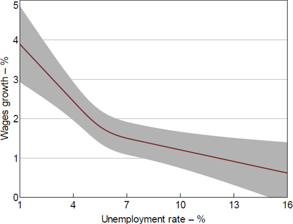
Notes: 95 per cent confidence intervals estimated using the Delta method; kinks set at 4.0, 5.5 and 7.5 per cent
Sources: ABS; Authors' calculations; National Skills Commission
Footnotes
With the exception of the additional spline terms, the model is the same as specification (B) in Table 2. [35]
Changes in the NAIRU and inflation expectations over time will shift the Phillips curve, but have no bearing on our conclusions as to its slope and curvature. When the unemployment rate is equal to the NAIRU, price inflation will be equal to long-run inflation expectations. However, with a positive rate of productivity growth, wages will grow at a faster rate than prices, all else being equal. [36]
See Dupont (2002) for a description of restricted cubic spline models. While we place the three kinks at the 23rd, 53rd and 80th percentiles (to be consistent with Figure 7), it is more common to place those kinks at the 10th, 50th and 90th percentiles. However, we find that our results are virtually unchanged when we adopt the 10–50–90 approach. [37]