RDP 2017-02: Anticipatory Monetary Policy and the ‘Price Puzzle’ 3. Robustness to Alternative Specifications
May 2017
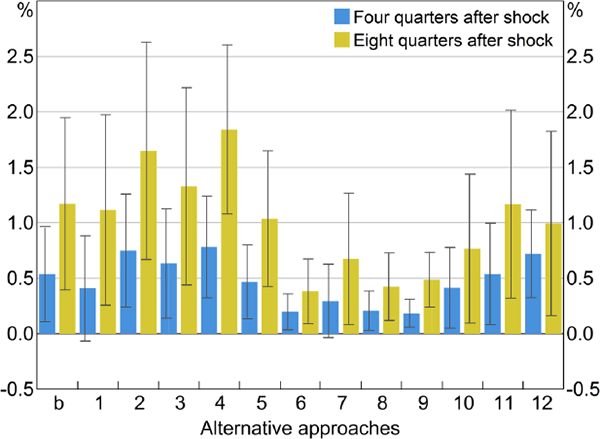
Because our baseline results for inflation were so surprising, we experimented with alternative specifications of the first-stage regression. We present 12 of these alternatives, together with our baseline labelled ‘b’, in Figure 7. These alternatives are briefly described below with further details where necessary in Appendix C. For the baseline and each of the 12 different specifications, the blue columns show estimated responses of the price level after four quarters to a 1 percentage point contractionary shock to monetary policy. Olive columns show responses after eight quarters and black lines show 90 per cent confidence intervals.

Notes: ADL model; blue bars show the cumulated response of inflation four quarters after a permanent 1 percentage point shock to the cash rate, using the 12 alternative approaches for constructing the cash rate shock; olive bars show the response after eight quarters, and black lines are 90 per cent confidence intervals; sample period for most estimates is 1994:Q2–2015:Q4, exceptions are: Approach 4, which begins in 1996; Approach 7, which begins in 2001; Approach 8, which begins in 1990; and Approach 9 which begins in 1988:Q3
Sources: ABS; Authors' calculations; Business Review Weekly; Consensus Economics; RBA
As explained earlier, our baseline only includes forecasts with a horizon out to two quarters ahead. Forecasts at longer horizons are more likely to be contaminated by the current month's policy decision and the assumed path of the cash rate going forward. However, policymakers often explain their decisions with reference to a longer-term outlook. Accordingly, our first alternative specification replaces the two-quarter-ahead forecasts for year-ended GDP growth and inflation in Equation (9) with four-quarter-ahead forecasts. Estimates are shown as Approach 1 in Figure 7.
In Approach 2 we replace the GDP forecasts with forecasts for the unemployment rate, which some argue are more relevant to the inflation outlook than the GDP growth forecasts. Extending the unemployment rate and inflation forecasts out to four quarters ahead (as in Approach 1) also gave similar results (not shown).
In Approach 3 we include the change in the cash rate announced at the previous month's Board meeting in the first-stage regression in order to allay concerns about serial correlation, interest rate smoothing or the omission of a persistent variable. In some estimated Taylor rules, this variable is highly significant.
As noted earlier, in the early and mid 1990s the Bank responded more aggressively than usual to the inflation outlook in order to reinforce credibility in the inflation target. Barakchian and Crowe (2013) argue that such changes in the weight on the forecasts in the central bank's reaction function could lead to misleading results. In Approach 4, we restrict our sample to begin in 1996:Q1, a period for which the coefficients on the policy rule were arguably more stable. The resulting series should identify a narrower set of monetary shocks, namely innovations to the policy rule rather than changes in the coefficients of the rule.
In Section 2 we showed that an unbiased estimate of the effect of the cash rate on inflation can be obtained by controlling for central bank inflation forecasts, and nothing else. Cochrane (2004) argues that this is more efficient than Romer and Romer's (2004) approach, since it purges policy of systematic anticipatory changes while retaining all other variations in the cash rate – including any responses to activity above and beyond its effect on the inflation outlook – to estimate the effect on inflation more precisely. Consistent with this argument, we control only for the inflation forecasts out to four quarters ahead in Approach 5.[13] Cochrane argues this ‘stripped down’ model is asymptotically equivalent to Romer and Romer's estimator (i.e. our baseline model). However, in small samples the approaches can and do yield different results.
We do not adopt Approach 5 as our baseline, preferring the approach of Romer and Romer (2004) and Cloyne and Hürtgen (2016), who also control for estimates of output growth and the unemployment rate. A rationale is that policymakers may react to inflation at longer horizons than included in our regression, or focus on alternative measures of inflation. If so, key determinants of inflation, such as the extra controls, may capture some anticipatory behaviour. This arguably reduces misspecification bias at a cost of some efficiency.
Approaches 1–5 follow the baseline in constructing shocks by using cash rate changes from forecast-month meetings. This omits 7 out of every 11 Board meetings each year, which reduces the variation in the cash rate and hence impairs the efficiency of our estimator. The rationale is that the economic outlook is not well described by official forecasts at other meetings, so a shock series that uses cash rate changes announced at those meetings may not adequately account for anticipatory policy. Furthermore, as noted above, the extra power is not necessary.
Approaches 6–9 relax these assumptions by using cash rate changes from all meetings. Whereas our baseline first-stage specification was estimated using only one observation per quarter, these four approaches use monthly data. Approach 6 explains monthly changes in interest rates since 1991 with the most recent official forecast. For example, the August SMP forecasts are used to explain decisions in August, September and October (rather than just the August decision, as in our baseline). The first-stage regression uses data from all Board meetings; we then sum the residuals that fall within a given quarter to derive a quarterly series of policy shocks. This is similar to the baseline approach of Cloyne and Hürtgen (2016).
As discussed in Section 2.1, SMP forecasts are finalised after Board decisions are announced and thus incorporate financial market and other reactions to the announcement. The next few alternatives use forecasts that are finalised before policy decisions are announced, in order to address this concern more explicitly.
Rather than using the Tulip and Wallace (2012) data for official forecasts, for Approach 7 we collect internal staff forecasts from the Bank's unpublished archives. In forecast months, these forecasts, shown in Figure 3, are those tabulated in the Board paper or presented to the Bank's internal Policy Discussion Group in the lead-up to the Board meeting. In other months, they are an archive of the forecasts made prior to the Board meeting. These forecasts are not official and often seem to reflect an incomplete incorporation of new data. They are not usually tabulated in the official Board papers and it is unclear the extent to which the information these forecasts contain is conveyed to the Board (in non-forecast-month meetings). Moreover, the archives are only available from 2001 onwards and have not been consistently maintained. Like Approach 6, we estimate the first-stage regression using interest rate changes from every Board meeting, rather than just the forecast-month meetings.
Rather than using the RBA's forecasts for quarterly underlying inflation and GDP growth, for Approach 8 we use Consensus Economics forecasts for year-ended growth in the headline CPI for the coming and following December quarter along with Consensus forecasts for year-average growth in GDP for the current and following calendar year (see Appendix C). Because Consensus forecasts are compiled around the middle of the month, we assign each set of forecasts to the following month's Board meeting. For example, we assign the survey conducted on 13 April 2015 to the Board meeting on 5 May 2015.[14] The Consensus data allow us to estimate the first-stage regression using data at a monthly frequency. This has similar advantages as Approach 7. One disadvantage is that Consensus forecasts imperfectly capture the central bank's forward-looking behaviour. In practice, however, Tulip and Wallace (2012) showed that Consensus forecasts have very similar properties to RBA forecasts. Cloyne and Hürtgen (2016, Section IV.C) find that their estimates for the United Kingdom using private sector forecasts are almost identical to estimates using Bank of England forecasts.
The specification we use in Approach 9 is the same as Approach 8, but extends the estimation sample for both the first- and second-stage regressions back to 1985:Q3 by incorporating data from the Business Review Weekly's quarterly survey of market economist forecasts. Using earlier data allows us to estimate policy effects with more precision, since policy shocks were much larger prior to the inflation-targeting era. In particular, it captures the high interest rates of the late 1980s, which were followed by a large reduction in inflation.
A third set of alternative specifications depart more fundamentally from the approach of Romer and Romer (2004) in that they do not use economic forecasts. In these specifications, we calculate policy ‘surprises’ using the daily changes in the bank bill interest rate around the policy announcements. Previous studies that have estimated macroeconomic effects of monetary shocks extracted from financial market data include Faust, Swanson and Wright (2004) and Barakchian and Crowe (2013). We consider measures based on both the 1-month (Approach 10) and 3-month (Approach 11) bank bill rates (see Appendix C). Lastly, Approach 12 considers the results if we use a shock series obtained from the recursive VAR in Figure 1.
As can be seen in Figure 7, every shock measure we consider generates a price puzzle. At a horizon of eight quarters, every response is significantly different from zero at the 10 per cent level. This highlights that the price puzzle in Australia is robust to a wide range of specifications designed to control for anticipatory policy.
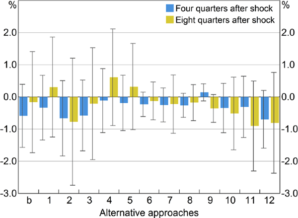
We show the sensitivity analysis for the effect of monetary policy on output in Figure 8. Our baseline estimates (i.e. those shown in Figure 6) are near the middle of the estimates from our 12 alternative specifications, most of which point to an effect that is ‘correctly’ signed but statistically indistinguishable from zero.

Notes: ADL model; blue bars show the cumulated response of real GDP four quarters after a permanent 1 percentage point shock to the cash rate, using the 12 alternative approaches for constructing the cash rate shock; olive bars show the response after eight quarters, and black lines are 90 per cent confidence intervals; sample period for most estimates is 1994:Q2–2015:Q4, exceptions are: Approach 4, which begins in 1996; Approach 7, which begins in 2001; Approach 8, which begins in 1990; and Approach 9, which begins in 1988:Q3
Sources: ABS; Authors' calculations; Business Review Weekly; Consensus Economics; RBA
3.1 VAR Model
Including our new measure of monetary shocks into a VAR permits an easier comparison with other studies. Unlike the six-variable VAR in Figure 1, we use a more parsimonious model that contains only real GDP (in levels), underlying inflation and our measure of monetary policy shocks (in that order). We do not include other variables because we have already isolated a policy shock in the first stage, so including variables such as the exchange rate will unnecessarily strip out useful variation from our measure of policy shocks. This is also closer to the specification used in Romer and Romer (2004). Because VARs are typically based on the cash rate in levels, we cumulate our measure of shocks over time.
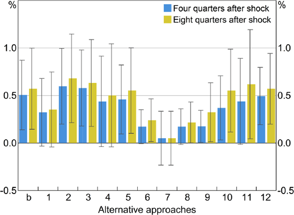
Figure 9 presents the impulse response functions (IRFs) of the price level to a temporary 1 percentage point shock to the cash rate. We present IRFs for both our ‘baseline’ shock series and our 12 alternative approaches. The policy experiment considered here involves a less persistent shock to policy than the permanent shock we simulated in the ADL model. Accordingly, while the responses of output and prices are qualitatively similar to the ADL models, they tend to be smaller and more transitory. Across most specifications we consider, a price puzzle is evident.

Notes: VAR model; Cholesky decomposition, with ordering: GDP, underlying inflation, cash rate shocks; blue bars show the cumulated response of inflation four quarters after a temporary 1 percentage point shock to the cash rate, using the 12 alternative approaches for constructing the cash rate shock; olive bars show the response after eight quarters, and black lines are 90 per cent confidence intervals; sample period for most estimates is 1991:Q2–2015:Q4, exceptions are: Approach 4, which begins in 1996; Approach 7, which begins in 2001; Approach 8, which begins in 1990; and Approach 9, which begins in 1988:Q3
Sources: ABS; Authors' calculations; Business Review Weekly; Consensus Economics; RBA
Footnotes
We also include revisions to the forecasts out to four quarters ahead. [13]
Assigning each Consensus forecast to the following month's Board meeting ensures that the forecasts do not capture information that would not have been available to the Board in real time (or the effect of the policy decision itself on the forecast). [14]