RDP 2015-15: Household Economic Inequality in Australia Appendix B: Alternative Survey Measures of Inequality

In this Appendix we adopt an alternative definition of imputed rent to cross-check the results for consumption and income inequality in the paper.

B.1 Hedonic Estimates of Imputed Rent

The alternative measure of imputed rent is calculated using the ABS hedonic modelling methodology, which estimates the market value of the rental equivalent for owner-occupied dwellings using the dwelling characteristics available in the HES.

The dependent variable is the logarithm of gross imputed rent for the sample of owner-occupier households.^[22] There are two types of explanatory variables in the model – Type I and Type II variables.

The Type I variables describe the characteristics of the dwelling, including:^[23]

• State
• Section of state (i.e. capital city or balance of state)
• Type of dwelling structure
• Number of bedrooms.

The Type II variables describe the households renting the dwellings, including:^[24]

• Household income
• Type of landlord (i.e. public or private landlord).

The model for market renters is:

where ln(R_i) is the natural logarithm of the weekly rent of household i, X_ij is the set of Type I variables and Z_ik is the set of Type II variables for each household, M_i is the estimated Inverse Mills ratio and ε_i is a normally distributed error term with a mean of zero and a standard deviation of σ.

The Inverse Mills ratio is calculated using the Heckman procedure. This adjusts for possible bias that could result from non-random selection. The Inverse Mills ratio is the ratio of the probability distribution function and the cumulative distribution function of the standard Z-score estimated in the probit model:

where X is a set of dwelling and household characteristics (e.g. age and educational attainment of household head) that determine whether a household rents or not.^[25]

Next, we make an adjustment to the intercept to control for the Type II variables. Specifically, the intercept is adjusted to the mean for renters:

where is the adjusted intercept for imputation, is the intercept estimate of the basic model, is the estimated coefficient for each Type II variable, and is the mean of each Type II variable.

A scaling factor is then applied to preserve the relationship between the observed and model rent estimates for private market renters. The imputed rent distribution is re-positioned to the original median rent observed in the private market renters' data.

and so:

where is the estimated gross imputed rent for owner-occupier household i.

Since the model does not fully explain the variation in rent for high-value dwellings, an extrapolation method is used to adjust gross imputed rent for high-value dwellings. A ceiling rent is determined by a visual inspection of the modelled results. The ceiling rent is divided by the estimated annual average rate of return for all owners. A regression model is fitted to owners below the house value cut-off:

where is the rental rate of return for owner-occupier household i and h_i is the value of that household's dwelling.

The gross imputed rent for owners with house values above the cut-off were recalculated using the statistically significant coefficients in the above equation. The extrapolated imputed rent is given by:^[26]

where is the adjusted gross imputed rent for the jth owner-occupied dwelling, p_j is the jth home value and is the estimated rental rate of return. For further details, see Australian Bureau of Statistics (2008).

B.2 Alternative Estimates of Inequality

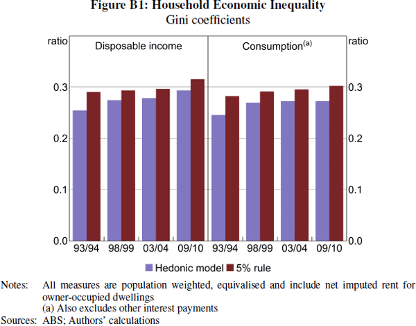
Using the alternative measure of imputed rent results in a lower level of inequality for both income and consumption (as measured by the Gini coefficient) compared with the simple approach in the main paper (Figure B1). The upward trend for disposable income inequality is apparent under both approaches. However, the rise in consumption inequality is less apparent under the hedonic modelling approach.

Footnotes

The explanatory variables used to estimate the market rent are not as extensive as those used by the ABS as we only have access to the basic confidentialised unit record files. [22]

Prior to the 2003/04 survey, the ‘section of state’ variable is not included. The ‘state’ variable is not included in the 1988/89 survey. [23]

Prior to the 2003/04 survey, landlord type is not included so we use tenure type to capture similar information. [24]

Prior to 1998/99, the education variable is not included. [25]

We are not able to use this extrapolation method for the 1975/76, 1984 and 1988/89 surveys because the estimated housing value of the dwelling is not included. [26]