RDP 2015-13: Seasonal Adjustment of Chinese Economic Statistics 3. Seasonally Adjusting Chinese Economic Time Series
November 2015 – ISSN 1448-5109 (Online)
- Download the Paper 1.18MB
This section discusses the properties of a selection of Chinese economic time series and shows the results of seasonal adjustment using X-12-ARIMA and SEATS.
3.1 Data
We consider one quarterly times series (GDP) and twelve monthly time series: fixed asset investment (FAI), industrial value added (‘industrial production’), the consumer price index (CPI), merchandise export values, merchandise import values, credit, total social financing (TSF), money supply (M2), crude steel gross output, rail freight volumes, power generation, and nominal retail sales. These data are all official statistics produced by the NBS, China Customs (exports and imports) or the People's Bank of China (credit, TSF and money supply). Table 1 displays some basic properties of the times series used.[9]
| Series | Source(a) | Sample | Units | Mean growth per annum(b) |
Standard deviation(c) |
|---|---|---|---|---|---|
| FAI | NBS | 2000:M1–2014:M2 | Values (CNY) | 27.7 | 8.8 |
| Industrial production | NBS | 2000:M1–2014:M2 | Index | 13.4 | 3.6 |
| CPI | NBS | 2000:M1–2014:M2 | Index | 2.4 | 2.3 |
| Exports | GAC | 2000:M1–2014:M2 | Values (USD) | 14.6 | 16.5 |
| Imports | GAC | 2000:M1–2014:M2 | Values (USD) | 16.9 | 19.5 |
| Credit | PBC | 2000:M1–2014:M2 | Values (CNY) | 16.9 | 5.2 |
| TSF | PBC | 2002:M2–2014:M2 | Values (CNY) | 20.6 | 91.2 |
| Money supply | NBS | 2000:M1–2014:M2 | Values (CNY) | 17.1 | 3.7 |
| Crude steel | NBS | 2000:M1–2013:M12 | Tonnes | 13.8 | 10.9 |
| Rail freight | NBS | 2000:M1–2014:M2 | Tonnes | 5.8 | 7.1 |
| Power generation | NBS | 2000:M1–2014:M2 | Kilowatt hours | 9.6 | 7.7 |
| Retail sales | NBS | 2000:M1–2011:M12 | Values (CNY) | 18.9 | 4.7 |
| Real GDP | NBS | 2000:Q1–2013:Q4 | Index | 9.9 | 2.0 |
|
Notes: (a) PBC refers to People's Bank of China, GAC refers to the General Administration
of Customs of the People's Republic of China (b) Compound geometric annual average of month-on-month percentage changes (quarter-on-quarter for quarterly data) (c) Standard deviation of year-on-year (year-ended) percentage changes Sources: Authors' calculations; CEIC Data |
|||||
A number of these series were chosen due to the intensive use that is made of them by analysts of Chinese macroeconomic developments (e.g. Batson 2013). Industrial production, FAI, retail sales, trade values, M2, credit and TSF are regularly reported in the press following their monthly releases. Holz (2013) and Fernald, Malkin and Spiegel (2013) find little evidence that Chinese official data are systematically distorted. However, given that many official data series are still viewed with scepticism by analysts, we also consider three less ‘high-profile’ series – crude steel, rail freight volumes and electricity generation – that are also timely indicators of growth in Chinese economic activity.[10]
We conduct adjustments for the moving holiday associated with Chinese New Year based on an historical identification of the scheduling of public holidays by government authorities (Table 2). There are currently seven official nationwide public holidays. These are: New Year (1 January), Chinese New Year (three days in January/February), the Qingming festival (4 or 5 April), Labour Day (1 May), the Dragon Boat festival (one day in May/June), the Mid-Autumn festival (one day in September/October) and National Day (1–3 October).
| Year | Date of first day | Public holidays | Additional work days |
|---|---|---|---|
| 2000 | 5 February | 4–10 February | 11–12 February |
| 2001 | 24 January | 24–23 January | 20–21 January |
| 2002 | 12 February | 12–18 February | 9–10 February |
| 2003 | 1 February | 1–7 February | 8–9 February |
| 2004 | 22 January | 22–28 January | 17–18 January |
| 2005 | 9 February | 9–15 February | 5–6 February |
| 2006 | 29 January | 29 January–4 February | 28 January, 5 February |
| 2007 | 18 February | 18–24 February | 17, 25 February |
| 2008 | 7 February | 6–12 February | 2–3 February |
| 2009 | 26 January | 25–31 January | 24 January, 1 February |
| 2010 | 14 February | 13–19 February | 20–21 February |
| 2011 | 3 February | 2–8 February | 30 January, 12 February |
| 2012 | 23 January | 22–28 January | 21, 29 January |
| 2013 | 10 February | 9–15 February | 16–17 February |
| 2014 | 31 January | 31 January–6 February | 26 January, 8 February |
|
Sources: Selected government releases and newspaper articles |
|||
The scheme of public holidays and working weeks in China has changed over time. The July 1994 Labor Law of the People's Republic of China stipulated a 44 hour working week, although this was shortened in March 1995 when the State Council issued a circular announcing the adoption of a 40 hour (five day) working week. Prior to 2000, a single day was observed as a public holiday for Chinese New Year. This was extended to three days in 2000 following the State Council's revision to the Regulation on National Festival and Commemorative Holidays in September 1999. In practice, from 2000 onwards the government has issued dates for these three days matching traditional dates of the Spring Festival on the Chinese lunar calendar. It has typically issued instructions lengthening the three-day holiday to a seven-day holiday by absorbing adjacent weekdays and requiring a prior, or subsequent, Saturday and Sunday to be treated as working days.
The sample we consider is, in general, 2000:M1–2014:M2 for monthly data and 2000:Q1–2014:Q1 for quarterly data.[11] Although earlier data are available for many series, we start the sample in 2000 due to the significant changes made to public holiday arrangements, which effectively initiated the practice of a week-long public holiday in observance of Chinese New Year. While the effects of Chinese New Year are clearly observable in unadjusted data prior to 2000, the seasonal pattern changes markedly in 2000. We exclude the sample prior to 2000 to prevent this major change in policy towards public holidays contaminating our estimated moving holiday coefficients.
Another, more minor, policy-driven change is also worth noting. In 2008, the Labour Day holiday was shortened from a three-day holiday (which was typically expanded to seven) to a one-day holiday. In place of the longer holiday, the traditional Dragon Boat, Qingming and Mid-Autumn festivals were all listed as one-day official public holidays. As with Chinese New Year, the Dragon Boat and Mid-Autumn festivals move between months on the Gregorian calendar. Also similar to Chinese New Year, these one-day holidays are usually extended to three days.[12]
In this analysis, we control for the effect of Chinese New Year, the Dragon Boat festival and the Mid-Autumn festival. Although the more recent, and shorter, moving holidays associated with the two smaller festivals have a smaller potential impact on economic activity, their importance cannot be ruled out ex ante.[13]
Finally, it is worth noting that our ability to make explicit adjustments for Chinese New Year is constrained by how the raw economic data are released. Industrial production and FAI figures are not released separately for January and February. Rather, a total figure for the two months is released at the same time as the February release for other statistics. As it is not possible to identify the value or volume of activity in each month separately, for these two series we assign the average monthly flow to each of the two months prior to seasonal adjustment.
3.2 Results
We use the X-13-ARIMA-SEATS program to conduct ARIMA modelling and seasonal adjustment, and the Genhol utility developed by Brian C Monsell to construct moving holiday regressors.[14] Table 3 summarises the results of ARIMA modelling for both X-12 and SEATS, and diagnostic tests for the presence of seasonality after the data have been adjusted. We refer to estimates obtained using these models as our ‘benchmark’ seasonal adjustment estimates. Figures for a number of these series are included for reference in Appendix C.
| Series | Seasonality detected | FS | FM | ARIMA model chosen |
SEATS ARIMA model used |
|---|---|---|---|---|---|
| FAI | Yes | 173.7*** | 1.5 | (0 1 1)(1 1 0) | Same |
| Industrial production | Yes | 80.0*** | 8.8** | (0 1 1)(0 1 0) | Same |
| CPI(a) | Yes | 125.3*** | 3.5* | (3 1 0)(0 1 1) | Same |
| Exports(a) | Yes | 106.9*** | 0.5 | (0 1 1)(0 1 1) | Same |
| Imports(b) | Yes | 63.6*** | 1.5 | (0 1 0)(0 1 1) | Same |
| Credit(c) | Yes | 29.1*** | 3.9** | (1 1 2)(1 0 1) | Same |
| TSF(a) | Yes | 52.0*** | 3.3** | (1 1 1)(0 1 1) | Same |
| Money supply(d) | Yes | 31.1*** | 2.6** | (0 1 0)(0 1 1) | Same |
| Crude steel | Yes | 11.1*** | 4.8** | (0 1 0)(0 1 1) | Same |
| Rail freight(a) | Yes | 35.1*** | 1.4 | (0 1 0)(0 1 1) | Same |
| Power generation(a) | Yes | 267.4*** | 1.9* | (0 1 1)(0 1 1) | Same |
| Retail sales(a) | Yes | 263.9*** | 5.5** | (0 1 0)(0 1 1) | (0 1 1)(0 1 1) |
| Real GDP | Yes | 55,630.1*** | 3.2** | (0 1 1)(0 1 0) | Same |
|
Notes: ***, ** and * represent significance at the 0.1, 1 and 5 per cent levels,
respectively (a) Adjusted for Chinese New Year (b) Adjusted for Chinese New Year, the Dragon Boat festival and Mid-Autumn festival (c) Adjusted for Chinese New Year and the Dragon Boat festival (d) Adjusted for Chinese New Year and the Mid-Autumn festival |
|||||
For all series an F-test for the presence of a seasonal pattern (FS) finds evidence of seasonality. Significant evidence of moving seasonality (FM) is also found for many series.[15] The ARIMA models chosen by the automatic model selection procedure for use in SEATS are largely the same as those to which X-12 filters are applied. With the exception of the X-12-ARIMA adjustment for FAI, visual analysis of spectral plots reveals no evidence of residual seasonality. We consider the case of FAI later.
Table 4 displays the estimation results for our moving holiday corrections. As noted earlier, due to data constraints we are unable to correct for Chinese New Year effects in the case of FAI and industrial production. Corrections for the Dragon Boat and Mid-Autumn holidays were also found to be insignificant for these series. GDP was not corrected for moving holiday effects as the Chinese New Year holiday always falls within the March quarter. Similarly, there was no evidence of significant moving holiday corrections for crude steel production.
| Series | Chinese New Year effect detected (p-value) | Dragon Boat festival effect detected (p-value) | Mid-Autumn festival effect detected (p-value) |
|---|---|---|---|
| CPI | Yes (0.00) | No (0.77) | No (0.40) |
| Exports | Yes (0.00) | No (0.43) | No (0.58) |
| Imports | Yes (0.00) | Yes (0.02) | Yes (0.02) |
| Credit | Yes (0.03) | Yes (0.00) | No (0.90) |
| TSF | Yes (0.00) | No (0.31) | No (0.58) |
| Money supply | Yes (0.00) | No (0.39) | Yes (0.03) |
| Rail freight | Yes (0.00) | No (0.59) | No (0.86) |
| Power generation | Yes (0.00) | No (0.12) | No (0.27) |
| Retail sales | Yes (0.00) | No (0.98) | No (0.82) |
With these exceptions, Chinese New Year was found to be significant in all cases. A significant effect of the Dragon Boat festival was found for imports and credit, and the Mid-Autumn festival was significant for imports and money supply.[16] The fact that not all holidays were statistically significant for all series suggests that different time series are affected by the various moving holidays to greater or lesser extents. This warns against a ‘one-size-fits-all’ approach to correcting for moving holidays in Chinese data.
Table 5 focuses more specifically on the results for our Chinese New Year moving holiday corrections.[17] A couple of observations can be made about the Chinese New Year corrections chosen by our benchmark procedure. First, the sub-period lengths found by the procedure tend to be relatively long, with most being longer than ten days. A consequence is that the data for March are often also affected by the Chinese New Year holiday when it falls late in February.
| Series | Chinese New Year effect detected | Chi-square (p-value) | Sub-period 1 | Sub-period 2 | Sub-period 3 |
|---|---|---|---|---|---|
| Number of days | |||||
| CPI | Yes | 153.8 (0.00) | 6 | 5 | 8 |
| Exports | Yes | 132.7 (0.00) | 11 | 19 | 20 |
| Imports | Yes | 235.5 (0.00) | 12 | 6 | 20 |
| Credit | Yes | 8.9 (0.00) | 3 | 17 | 18 |
| TSF | Yes | 34.9 (0.00) | 19 | 20 | 15 |
| Money supply | Yes | 13.3 (0.01) | 11 | 20 | 3 |
| Rail freight | Yes | 23.7 (0.00) | 13 | 20 | 8 |
| Power generation | Yes | 656.0 (0.00) | 12 | 5 | 17 |
| Retail sales | Yes | 73.5 (0.00) | 10 | 16 | 3 |
A second observation is that the benchmark sub-period lengths vary considerably across different time series. This suggests that there may be a benefit in allowing each of the three sub-periods to vary for different time series, rather than choosing a length in ad hoc fashion that applies to all three intervals. However, there is some evidence that applying sub-period lengths that are shorter than preferred by our procedure can give an adjustment that appears inadequate upon visual inspection, whereas the results are not usually substantially changed by applying sub-period lengths that are longer.
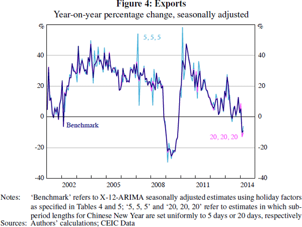
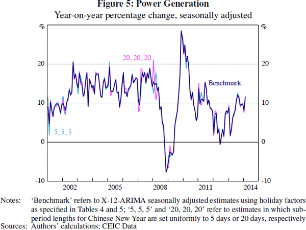
Figures 4 and 5 show sensitivity results for exports and power generation. In each case, applying sub-periods shorter than preferred by our procedure increases the volatility of the year-on-year growth rates noticeably around Chinese New Year. For exports, applying longer sub-period lengths makes little difference to the results. But in the case of power generation, longer sub-periods also result in sharp movements in year-on-year growth rates around Chinese New Year. Given that the sub-periods chosen by our procedure vary noticeably across the indicators we have selected, it seems unlikely that a uniform set of sub-periods – that is, τi = τ, as suggested in earlier literature – will adjust for Chinese New Year adequately across all series.
As our procedure requires some computation, it is worth comparing these results to those of simpler approaches. One of the most widely reported methods of assessing momentum in Chinese economic data is to use the year-on-year percentage change. Computing year-on-year percentage changes is a simple way of attempting to abstract from seasonal effects. However, when a moving holiday is present there are typically very sharp movements in the year-on-year growth rate during the months in which the holiday can occur.
A good example is power generation. Since many factories and offices close down over the Chinese New Year holiday period, electricity generation typically declines. If Chinese New Year occurs in January one year and in February the following year, then year-on-year growth in power generation tends to spike sharply higher in January of the second year and sharply lower in February. This effect can be seen in the non-seasonally adjusted line in Figure 6. An observer would obtain little information about the momentum in Chinese power generation around the time of Chinese New Year using this approach.
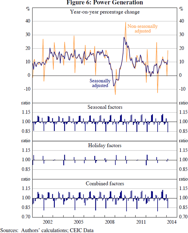
The influence of Chinese New Year can clearly be seen in the seasonal decomposition of the power generation series produced by X-12-ARIMA (Figure 6). Power generation has a fairly predictable seasonal pattern (second panel of Figure 6), abstracting from Chinese New Year. Incorporating Chinese New Year, the pattern is noticeably less regular (bottom panel of Figure 6).
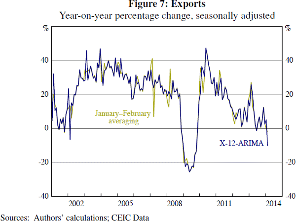
Another simple method of abstracting from Chinese New Year is to average the values for January and February. By construction, this method will remove the Chinese New Year effect from these months at the cost of also removing some dynamic variation from the series. Moreover, this method gives less timely information than alternative approaches, since a reading on momentum in a given series cannot be obtained until the February data are released. A further potential problem with this approach is suggested by the results in Table 5. Because the effect of Chinese New Year spills over into March, January–February averaging prior to regular seasonal adjustment of the series may not account adequately for such spillovers.
The result of not accounting for a spillover of the moving holiday effect into March can be considered using the example of Chinese exports (Figure 7). The optimised sub-period lengths for the exports series are 11, 19 and 20 days for the periods before, during and after Chinese New Year. This pattern implies that the seasonal adjustment procedure will make a moving holiday correction for March. January–February averaging, however, makes no such adjustment, increasing the volatility of the adjusted series in some periods. For example, in 2007 (when the Chinese New Year holiday began on 18 February) a sharp drop can be seen in the year-on-year growth rate of the January–February averaged series in the month of March.
A general alternative to seasonal adjustment procedures such as X-12-ARIMA and SEATS is to regress the log of the original times series on deterministic monthly seasonal dummies. An advantage of this approach is its simplicity and transparency. The approach is widely used in the academic literature on China (e.g. Marquez and Schindler 2007; Cheung et al 2012). Figure 8 illustrates the results of this approach for the credit series. To ensure comparability with the X-12-ARIMA estimates, we incorporate the same Chinese New Year dummies in the estimation as specified in Table 5.
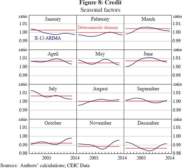
It is apparent from Figure 8 that the seasonal factors given by X-12-ARIMA can change noticeably over the sample, compared with the static factors produced by the deterministic dummy variable approach.[18] For example, seasonal factors that scale bank credit have varied significantly over time. In a rapidly changing developing economy, such as China, it appears inappropriate to assume that seasonal factors are constant.
3.3 X-12-ARIMA Versus SEATS
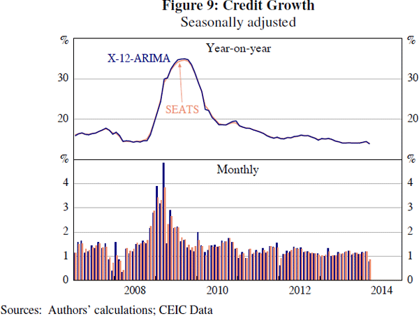
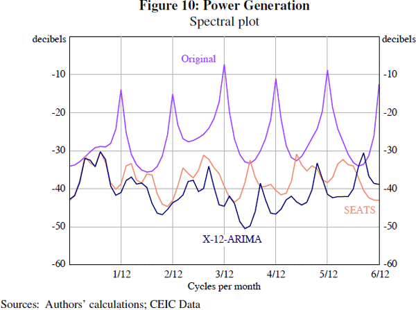
Our results suggest that neither SEATS nor X-12-ARIMA consistently outperforms the other. This is similar to the findings of previous work (Scott, Tiller and Chow 2007). For most indicators we consider, there is little difference: for example, the adjusted credit series is very similar outside of periods of great volatility in credit such as 2009 (Figure 9). Spectral plots generally suggest that both X-12-ARIMA and SEATS do an adequate job of seasonal adjustment, as suggested by the example of power generation (Figure 10). In both cases, peaks in the spectral density at the seasonal frequencies (highlighted by vertical lines in the figure) are eliminated by seasonal adjustment.[19]
Visual inspection of the other time series we consider suggests that only FAI and industrial production yield significant differences between the estimates produced by X-12-ARIMA and those produced by SEATS. These differences can be clearly seen in plots of the spectrum for FAI (Figure 11). It is apparent that the X-12 filter-based method is not adequately adjusting for seasonal effects, since there is a peak in the spectral plot of the seasonally adjusted series at one of the monthly seasonal frequencies (namely, the 1/12 cycles per month frequency). By comparison, the SEATS adjustment does not show any evidence of residual seasonality.
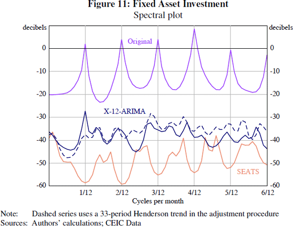
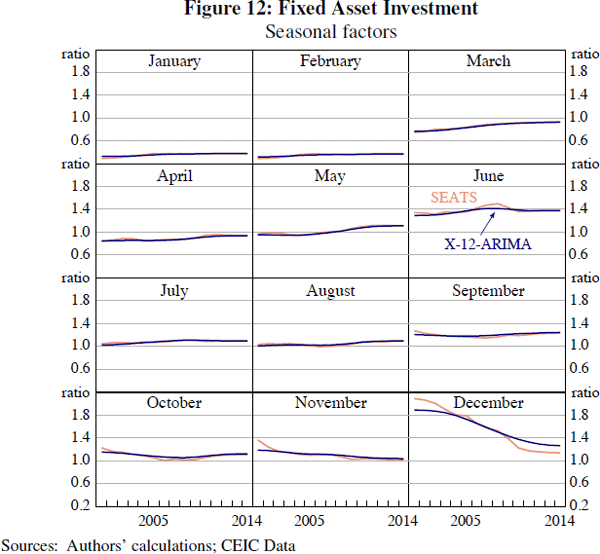
The better performance of SEATS for this series probably reflects the greater flexibility that SEATS has in selecting appropriate filters for seasonal adjustment. The seasonal decompositions of FAI provided by the two procedures indicate that SEATS estimates a much smoother trend than X-12-ARIMA.[20] Consequently, the seasonal factors are smoother under X-12-ARIMA. For both approaches, the December seasonal factor has become smaller over time (that is, closer to 1.0), with X-12-ARIMA estimating a smoother decline (Figure 12). But using a much smoother Henderson trend in the X-12 procedure (for example, a 33-period Henderson trend) allows X-12-ARIMA to estimate trend and seasonal components that are closer to those produced by SEATS, and greatly reduces the size of the seasonal peak in the spectral plot (see the dashed line in Figure 11). These results suggest that, for some series, the additional flexibility of the SEATS filter allows it to provide a better seasonal adjustment than the default filters used by X-12-ARIMA.
3.4 An Alternative Specification of Chinese New Year Corrections
Our benchmark approach to correcting for Chinese New Year allows the sub-period lengths (τ1,τ2,τ3) to be determined entirely by the data. A potential criticism of this approach is that we do not use all available information about Chinese public holidays. In particular, we identify the start of the second sub-period using the official start date for the Chinese New Year public holiday, but allow the length of the middle sub-period to be data-determined rather than incorporating the official end date of the public holiday into our calculations.
An alternative way of specifying the Chinese New Year holiday corrections is to fix the middle sub-period (τ2) for all series to a certain number of days, and allow the other two sub-periods (τ1 and τ3) to be decided with reference to the AICC. As the public holiday involves a total break from work of seven days, we set τ2 = 7.[21]
Table 6 shows the effect on the sub-period lengths chosen by our procedure. For the series considered, constraining the middle sub-period to seven days tends to result in longer ‘before’ and ‘after’ sub-periods than would otherwise be the case (compare Table 5).
| Series | Chinese New Year effect detected | Chi-square (p-value) | Sub-period 1 | Sub-period 2 | Sub-period 3 |
|---|---|---|---|---|---|
| Number of days | |||||
| CPI | Yes | 156.49 (0.00) | 7 | 7 | 11 |
| Exports | Yes | 125.48 (0.00) | 10 | 7 | 14 |
| Imports | Yes | 189.22 (0.00) | 7 | 7 | 3 |
| TSF | Yes | 19.17 (0.00) | 19 | 7 | 20 |
| Money supply | Yes | 9.43 (0.02) | 19 | 7 | 5 |
| Rail freight | Yes | 30.11 (0.00) | 18 | 7 | 20 |
| Power generation | Yes | 512.40 (0.00) | 12 | 7 | 16 |
| Retail sales | Yes | 62.36 (0.00) | 11 | 7 | 20 |
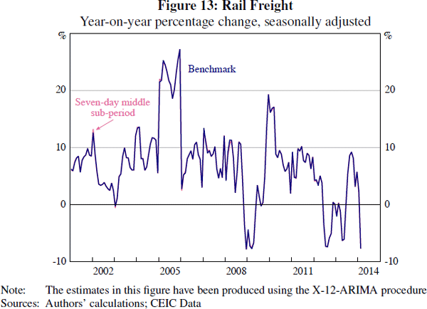
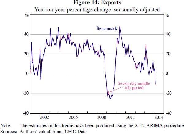
Fixing the middle sub-period affects all series differently, but usually has a limited effect on the overall seasonal adjustment. Figures 13 and 14 compare the results of the constrained holiday moving corrections to those of our benchmark approach for the rail freight and export series. For rail freight, and some other series, there is little discernible difference between the two approaches. For exports, the effect of fixing the middle sub-period can occasionally be seen around January–February. As there is no obvious criterion for choosing between the two approaches, we focus on the benchmark seasonally adjusted estimates.
3.5 Sensitivity Analysis
We consider the sensitivity of our benchmark seasonal adjustment to changes in sample with the aid of revision histories and sliding spans. The seasonal adjustment is more robust for some series than for others. The time series for which revisions are most noticeable are FAI, exports, imports and crude steel (Table 7). Interestingly, the X-12-ARIMA adjustment for FAI seems particularly prone to revision. This may reflect a poor seasonal adjustment for this series, consistent with the evidence from spectral plots.
| Series | X-12-ARIMA | SEATS |
|---|---|---|
| FAI | 2.59 | 1.04 |
| Industrial production | 0.47 | 0.60 |
| CPI | 0.10 | 0.08 |
| Exports | 1.50 | 1.48 |
| Imports | 1.86 | 1.73 |
| Credit | 0.25 | 0.28 |
| TSF | 0.13 | 0.10 |
| Money supply | 0.21 | 0.17 |
| Crude steel | 1.40 | 1.16 |
| Rail freight | 0.86 | 0.79 |
| Power generation | 0.62 | 0.59 |
| Retail sales | 0.41 | 0.47 |
| Real GDP | 0.13 | 0.24 |
Sliding spans analysis yields similar results. For each indicator, month-on-month changes in the seasonally adjusted series are compared over four overlapping spans (quarter-on-quarter changes are considered in the case of GDP). Table 8 shows the distribution of differences across spans. The seasonal adjustment for the trade, rail freight and crude steel data are least stable, while FAI does not stand out on this metric.
| Series | Span length | Minimum | Median | Maximum | Standard deviation |
|---|---|---|---|---|---|
| FAI | 86 | 0.00 | 0.25 | 1.77 | 0.37 |
| Industrial production | 86 | 0.01 | 0.36 | 2.12 | 0.53 |
| CPI | 98 | 0.00 | 0.08 | 0.26 | 0.12 |
| Exports | 99 | 0.02 | 1.09 | 3.31 | 1.61 |
| Imports | 99 | 0.02 | 1.22 | 3.29 | 1.81 |
| Credit | 102 | 0.01 | 0.11 | 0.65 | 0.17 |
| TSF | 98 | 0.01 | 0.13 | 0.45 | 0.19 |
| Money supply | 102 | 0.00 | 0.16 | 0.66 | 0.24 |
| Crude steel | 84 | 0.02 | 0.76 | 5.61 | 1.13 |
| Rail freight | 98 | 0.01 | 0.89 | 5.86 | 1.32 |
| Power generation | 98 | 0.03 | 0.51 | 2.54 | 0.75 |
| Retail sales | 84 | 0.03 | 0.45 | 1.84 | 0.67 |
| Real GDP(a) | 29 | 0.04 | 0.10 | 0.48 | 0.15 |
| Note: (a) Differences in quarter-on-quarter changes across spans | |||||
Footnotes
For additional information on the data used, see Appendix A. [9]
Some analysts have considered the ‘Li Keqiang Index’ (named after China's current premier) as an alternative gauge of economic activity. According to a US State Department memorandum released by WikiLeaks, in 2007 Mr Li Keqiang (then the Chinese Communist Party Secretary of Liaoning province) expressed scepticism about official statistics and noted his personal preference for data on railway cargo volumes, electricity consumption and bank credit (see Fernald et al (2013)). [10]
Owing to breaks in the NBS's provision of monthly data for retail sales after 2011, we only use monthly data up to December 2011 for this series. Similarly, due to a break in early 2014 we use crude steel data up to December 2013. [11]
If adjacent to a weekend a long weekend is observed; if not, a three-day holiday is mandated with one or two weekend days converted to working days to ensure a continuous three-day break from work. [12]
In practice, the Mid-Autumn festival coincides with the week-long National Day holiday in October around once every three years. When it does coincide, the authorities typically lengthen the National Day holiday by one day. [13]
These programs are available at <https://www.census.gov/srd/www/x13as/> and <https://www.census.gov/srd/www/genhol/>. The algorithm for optimising the sub-period lengths for moving holiday regressors described in Section 3 executes the X13-ARIMA-SEATS and Genhol programs iteratively until the AICC is minimised and the selection of a seasonal ARIMA model with optimised moving holiday corrections is completed. [14]
These tests are described in Appendix B, and are available for X-12-ARIMA output. Lothian and Morry's (1978) combined F-test for identifiable seasonality, which is reported as ‘M7’ by the X-12-ARIMA package output, also fails to reject the null hypothesis for most series, with the exception of crude steel which is found to be borderline. The results of such tests should be viewed with caution, as Lytras, Feldpausch and Bell (2007) have found that their power is typically quite low. [15]
The only series for which all three moving holidays were found to be significant was imports. While statistically significant, the Mid-Autumn festival dummies for this series were too small to be economically significant. [16]
Similar results are available for other moving holiday corrections but are omitted for brevity. [17]
The results of F-tests reported in Table 3 and additional figures in Appendix C provide evidence of moving seasonality for several other series. [18]
For spectral plots shown in this paper, we use estimated autoregressive spectral densities, following the advice of Findley et al (1998). The spectrum depicted in Figure 10 is reported in decibel (10log10) units on the vertical axis to compress the scale of the diagram for easy inspection. Frequencies 1/12 to 6/12 are shown on the horizontal axis. Intuitively, if an event occurs every six months, we would expect to see one-sixth of the cycle every month, and spikes at the 1/6 and 1/12 frequencies in the original data. [19]
This point was originally suggested to us by Hao Wang. [20]
In their application of the Lin and Liu (2003) Chinese New Year corrections, PBC (2006, p 391) propose the dummy variable specification (τ1 = 20,τ2 = 7,τ3 = 20). [21]