RDP 2013-04: Home Prices and Household Spending 2. Data
April 2013 – ISSN 1320-7229 (Print), ISSN 1448-5109 (Online)
- Download the Paper 732KB
2.1 The HILDA Survey Data
The HILDA Survey is a nationally representative annual household panel. It began in 2001 with around 7,700 responding households. It asks questions regarding families, household financial conditions, employment and wellbeing. Special modules provide another layer of detailed household-level information on household wealth every four years. In this study we use the household wealth modules of 2006 and 2010, which allow the dynamics of households' net worth to be examined at the component level.
We use three panels of responding households over the period 2003 to 2010. Panel one comprises households that did not split into different households over the sample and responded to the survey every year from 2003 to 2010 while maintaining their home tenure type (i.e. renter or homeowner).[4] The criteria for selection into panel one are detailed in Table 1: from an average responding sample of around 7,100 households each year we are left with a balanced panel of 1,947 households over eight years, for a total of 15,576 observations. Panel two drops renters from panel one. Panel three drops homeowners that moved house during the sample period from panel two, leaving us with 9,416 observations on stable home-owning households that provide a self-assessed home price for the same property in every wave of the survey. This sub-sample is of interest because housing transactions may be associated with higher spending if homeowners purchase goods and services when they move home. Moving home also provides an easy opportunity to add or reduce housing equity.
| Number of observations | ||
|---|---|---|
| Dropped | Remaining | |
| Criteria for selection into panel one – households | ||
| Responded in any given year | 57,027 | |
| Responded in all waves without household splitting | 37,395 | 19,632 |
| Did not change home tenure type | 3,840 | 15,792 |
| Born after 1919 and before 1981 | 216 | 15,576 |
| Sample size | 15,576 | |
| Criterion for selection into panel two – homeowners | ||
| Homeowner | 2,752 | 12,824 |
| Sample size | 12,824 | |
| Criterion for selection into panel three – non-moving homeowners | ||
| Did not move | 3,408 | 9,416 |
| Sample size | 9,416 | |
|
Sources: HILDA Release 10.0; authors' calculations |
||
Demographic variables considered are the age of the household head (the person most likely to make financial decisions for the household), number of children and adults in the household, education, occupation, region of residence and labour force status. The distribution of these variables for our panel of responding, non-splitting but possibly moving homeowners (panel two) is shown in Table A1.
The notion that young homeowners are likely to be more credit constrained than older homeowners is crucial to the interpretation of our results. This argument is supported by the cross-tabulations in Figure 2, which show the mean ratios of home loans to home prices and the mean ratios of unsecured credit card debts to home prices for panel two (homeowners). Younger homeowners have both high secured and unsecured debt, relative to older homeowners. Given that unsecured debt is likely to be more costly, this suggests that younger homeowners are on average more credit constrained than older homeowners. If younger homeowners were not credit constrained, one would expect them to substitute costly unsecured debt for less costly secured debt, and therefore the right-hand panel of Figure 2 to show no clear age pattern. An alternative, self-assessed, measure of credit constraints available within HILDA – the ability to raise $3,000 in an emergency – is also significantly positively correlated with age.[5]
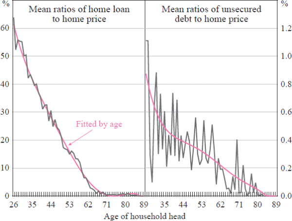
Notes: Calculated using all homeowners in panel two, defined in Table 1; fitted line obtained by regressing ratios on a polynomial in age; mean ratios of home loan to home price calculated over 2003 to 2010; mean ratios of unsecured debt to home price calculated using the wealth module years 2006 and 2010
Sources: HILDA Release 10.0; authors' calculations
The finding that young homeowners have high levels of secured and unsecured debt relative to the price of their homes is important. Disney et al (2010) find that only a sub-sample of homeowners with both high unsecured and secured debt increase their indebtedness (to potentially fund spending) following a rise in housing prices. Figure 2 shows that these homeowners are more likely to be young. The intuition behind the Disney et al (2010) result is straightforward: an increase in home prices allows a household to refinance – by substituting relatively expensive unsecured debt for secured debt – and potentially borrow more to spend.
The main household financial variables used in this study are self-reported non-housing expenditure and self-reported home prices. These data are discussed in the next two sections.
2.2 The HILDA Spending Estimates
The sample covers the period 2003 to 2010. Over this period, the ratio of HILDA non-housing spending to Australian Bureau of Statistics (ABS) final consumption expenditure has been steady at around one-half, and the relationship between movements in the HILDA spending numbers and the aggregate consumption figures has also been broadly stable with a correlation coefficient between the growth rates in these series of around 0.7 (Table 2).[6]
| 2003 | 2004 | 2005 | 2006 | 2007 | 2008 | 2009 | 2010 | |
|---|---|---|---|---|---|---|---|---|
| HILDA | 40,762 | 40,855 | 41,862 | 42,085 | 43,237 | 43,498 | 41,136 | 42,907 |
| ABS | 78,083 | 79,949 | 81,807 | 82,741 | 85,233 | 87,403 | 84,548 | 84,834 |
| Ratio | 0.52 | 0.51 | 0.51 | 0.51 | 0.51 | 0.50 | 0.49 | 0.51 |
|
Notes: 2009/10 dollars; deflated using trimmed mean CPI; HILDA data are from panel two Sources: ABS; HILDA Release 10.0; authors' calculations |
||||||||
Over the period 2006 to 2010, the HILDA spending estimates were calculated as the sum of the 25 self-reported spending categories defined according to the usual amount spent on weekly, monthly and annual items. However, from 2003 to 2005 self-reported figures are only available for three components: meals eaten out, groceries and childcare costs. The relationship between real spending on these items, the age of the household head and real total expenditure in the years 2006 to 2010 was used to impute real total spending for households from 2003 to 2005 (with the imputation adjusted for each panel). The estimated imputation regressions for panel two are presented in Table 3, where total spendingit is real total spending by household i in time t, meoit is real spending on meals eaten out, groit is real spending on groceries, ccit is real spending on childcare costs and ageit is the age of the household head. The first column shows the estimated coefficients from a linear specification, and the second column reports the estimated coefficients from a log-linear specification. Based on the fit, the log-linear model was chosen to impute spending in years 2003 to 2005. The fit of this regression, with an R2 of around 0.5, is consistent with other papers implementing a similar imputation method (see, for example, Skinner (1989); Lehnert (2004); and Contreras and Nichols (2010)).
| Linear model | Log-linear model(a) | |
|---|---|---|
| Meals eaten out | 4.06*** | 0.74*** |
| Groceries | 2.07*** | 0.52*** |
| Childcare costs | 0.2 | 0.05*** |
| Age | 762.7*** | 0.029*** |
| Age squared | −9.03*** | −0.0003*** |
| Constant | 805.57 | 9.3*** |
| Obs (2006–2010) | 8,015 | 8,015 |
| Adj R2 | 0.33 | 0.53 |
|
Notes: 2009/10 dollars; deflated using trimmed mean CPI; regression output
above is for panel two; ***, ** and * indicate significance at the 1,
5 and 10 per cent level, respectively Sources: HILDA Release 10.0; authors' calculations |
||

Restricting our spending variable in the analysis that follows to only the three items available over the period 2003 to 2010 does not change our qualitative results, although estimated wealth effects are smaller. The results are also robust to restricting the sample to the period 2006 to 2010.
2.3 HILDA Self-reported Home Prices
The home price variable used throughout this analysis is a household's self-reported home price every year from 2003 to 2010.[7] To check the consistency of these self-reported home prices with the aggregate data one can compare the mean of all self-reported home prices in each period to an independent nationwide measure (Table 4). The series appear to move together closely, albeit with a level difference; the correlation coefficient between the growth rates in each series is around 0.6. There is, however, one notable exception: the self-reported home price series misses the decline in nationwide prices that occurred between 2008 and 2009.
| 2003 | 2004 | 2005 | 2006 | 2007 | 2008 | 2009 | 2010 | |
|---|---|---|---|---|---|---|---|---|
| HILDA(a) | 370 | 417 | 438 | 466 | 498 | 522 | 536 | 574 |
| Independent(b) | 316 | 352 | 371 | 404 | 446 | 462 | 441 | 517 |
| Ratio | 1.17 | 1.19 | 1.18 | 1.15 | 1.11 | 1.13 | 1.21 | 1.11 |
|
Notes: (a) Unweighted mean from panel two Sources: ABS; HILDA Release 10.0; RBA; authors' calculations |
||||||||
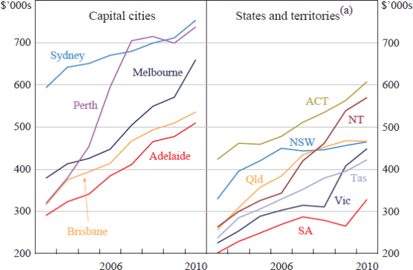
Figure 3 plots the mean of self-reported home prices within 12 major statistical regions identified in HILDA. These show large variations over time, across cities, and between capital cities and regions.
Note: (a) States exclude respective capital city
Sources: HILDA Release 10.0; authors' calculations
Footnotes
For example, if between 2009 and 2010 the adult membership of a household changed due to divorce there would be two households with the same 2009 household identification number in the 2010 dataset. Because divorce is often associated with financial stress and a fall in income, this could result in a changing pattern of consumption for both households. Accordingly, we drop these households from the sample. [4]
Arguably the best test of the credit constraints hypothesis would be to examine differences in home-price wealth effects for homeowners who could raise $3,000 in an emergency versus homeowners who could not raise $3,000 in an emergency. Unfortunately, non-response rates for this particular question are quite high. It is also difficult to control for a household's selection into subjective self-assessed categories. For these reasons, even the positive correlation between credit constraints and age reported in the text should be treated with some caution. [5]
In these comparisons, the ABS figures are not adjusted to make them more comparable to the HILDA Survey measure. However, differences in the concept and scope of these data should be borne in mind. The ABS data constitute the broadest, accruals-based measure, while the survey data measure only regular and recurring spending. Aside from these differences, notable omissions from the HILDA spending data include: entertainment expenses, non-fee education expenses, gifts and donations, personal and household services, health and beauty products, ornaments, art and jewellery, and financial service charges. [6]
Although we refer to home prices throughout, the data collected by the HILDA Survey are in fact on home values, and so will include changes in home values due to capital improvements as well as changes in home values due to pure price movements. [7]